7.1. AMET on AWS

The Atmospheric Model Evaluation Tool (AMET) (Appel et al., 2011) matches the model output for particular locations to the corresponding observed values from one or more networks of monitors using the program sitecmp, a post-processing routine from CMAQ. These pairings of values (model and observation) are then used to statistically and graphically analyze the model’s performance.

AMET Website helps users generate and view plots created by AMET R programs using a web browser.

Select projects, species, observational networks and programs to run using the interactive website with check box, and pull-down menu options. Create plots by selecting one or more observation networks and species, and select the program to run. Click on the Run Program button to run the program for the selected observation network and species on the VM. The R program queries the database, creates the plots, and provides links for the user to view either a pdf or png or html (for interactive plots) version of each plot.

Multiple programs are available to choose from for each plot type including Scatter Plots, Time Series Plots, Spatial Plots, Box Plots, Stacked Bar Plots, Kelly Plots, and Soccer Plots.

Programs that use Plotly are interactive, allowing you to subset the time range, and enable or disable items displayed on the plot by clicking on them in the legend.

Some programs also support model to model comparisons by selecting multiple projects, and also support display of results from multiple observation networks, and for multiple species on the same plot.

Link to AMET User Guide

7.1.1. Learn how to use AMET on AWS

• Create a VM with preloaded AMET databases and projects

• Perform analysis of the 3 MET projects (mcip, wrf, mpas) provided using the AMET Met Website

• Perform analysis using the AQ project aqExample and 18 EQUATES projects using the AMET AQ Website

• Load model data and observation data for a new project

• Troubleshoot and avoid errors

7.1.2. Databases and Projects Available

Database: amet

Projects | Click to expand!

AIR QUALITY
1. aqExample CMAQv5.5 test case July 2018, 12US1 (459x299x35)

METEOROLOGY
1. metExample_mcip, MCIP Test Case July 2016, 12US1 (459x299x35)
2. metExample_wrf, WRF Test Case July 2016, 12US1 (472x312x36)
3. metExample_mpas, MPAS Test Case July 2016, Globally-uniform 120 km resolution mesh

Database: amad_EQUATES

EQUATES: EPA’s Air QUAlity TimE Series Project

Projects | Click to expand!

Air Quality
1. CMAQv532_12US1_2002, 12US1 (459x299x35)
2. CMAQv532_12US1_2003, 12US1 (459x299x35)
3. CMAQv532_12US1_2004, 12US1 (459x299x35)
4. CMAQv532_12US1_2005, 12US1 (459x299x35)
5. CMAQv532_12US1_2006, 12US1 (459x299x35)
6. CMAQv532_12US1_2007, 12US1 (459x299x35)
7. CMAQv532_12US1_2008, 12US1 (459x299x35)
8. CMAQv532_12US1_2009, 12US1 (459x299x35)
9. CMAQv532_12US1_2010, 12US1 (459x299x35)
10. CMAQv532_12US1_2011, 12US1 (459x299x35)
11. CMAQv532_12US1_2012, 12US1 (459x299x35)
12. CMAQv532_12US1_2013, 12US1 (459x299x35)
13. CMAQv532_12US1_2014, 12US1 (459x299x35)
14. CMAQv532_12US1_2015, 12US1 (459x299x35)
15. CMAQv532_12US1_2016, 12US1 (459x299x35)
16. CMAQv532_12US1_2017, 12US1 (459x299x35)
17. CMAQv532_12US1_2018, 12US1 (459x299x35)
18. CMAQv532_12US1_2019, 12US1 (459x299x35)

7.2. Spin up a server using pre-installed AMET AMI

Note, the AMI is currently private, and only available upon request. Please send an email if you would like to be a beta-tester.
Send Email

• Select AMI named AMETv1.6_web that contains the AMETv1.6 installation with all data for MET and AQ loaded into database

• Select Launch instance from AMI

• Select Instance Type t3.xlarge (4vcpu and 16 GB memory) or t3.large (2 vcpu 8 GB memory)

• Select key pair

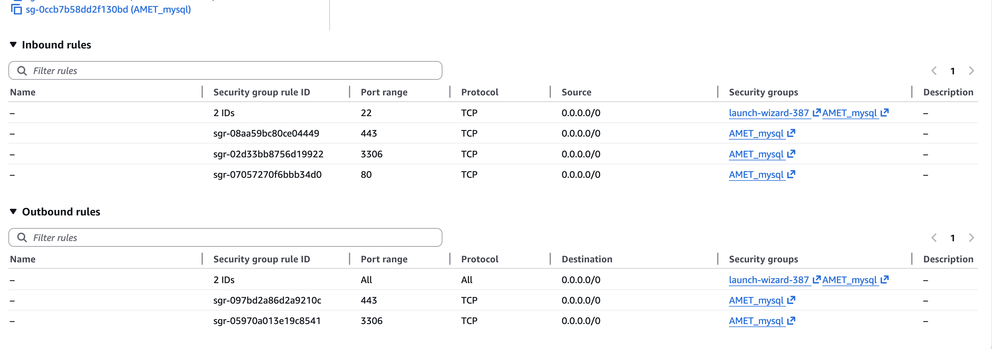
• Select existing security group - AMET_mysql

• AMET_mysql security group contains permissions for port 443 and 3306 for inbound and outbound open to all or restricted to your IP address or you can add these permissions when you launch a new instance from the AMI.

7.2.1. EC2 Instance Type Cost

T3 instance type, physical processor: Intel Skylake E5, CPU Architecture: x86_64

EC2 Instance Type	# vCPUs	Memory	Cost/hour	Cost/day
t3.2xlarge	8	32GB	$.33	$7.92
t3.xlarge	4	16GB	$.166	$3.98
t3.large	2	8GB	$.083	$1.99

7.2.2. Storage type costs

A 500 GiB AWS gp3 EBS volume typically costs $40.00 per month for storage alone ($0.08 per GiB-month) 3,000 IOPS & 125 MB/s throughput free

The Amazon Machine Image (AMI) with 500 GB of storage, which relies on EBS snapshots, typically costs $25.00 per month ($0.05 per GB-month) in the US East region

7.2.3. Login to the EC2 instance

 ssh -Y -i ./<your_pem_name>.pem ubuntu@xx.xx.xx

Edit the apache2 ports.conf file to specify the private IP address for the EC2 instance that is being used to run AMETv1.6

sudo vi /etc/apache2/ports.conf

cat /etc/apache2/ports.conf 

Output:

#If you just change the port or add more ports here, you will likely also
# have to change the VirtualHost statement in
# /etc/apache2/sites-enabled/000-default.conf

Listen 80
Listen 172.31.16.32:443
#Listen 3306

<IfModule ssl_module>
        Listen 443
</IfModule>

<IfModule mod_gnutls.c>
        Listen 443 
</IfModule>


<VirtualHost 172.31.16.32:443>

## This first-listed virtual host is also the default for *:80

ServerName http://localhost

DocumentRoot /var/www/html
</VirtualHost>

After the file is edited to use the private ip address, then restart the apache web server.

sudo systemctl restart apache2

7.2.4. Start the mariadb

sudo systemctl start mariadb

7.2.5. Check the version of mariadb that was installed

SELECT VERSION(); +———————————–+ | VERSION() | +———————————–+ | 10.11.13-MariaDB-0ubuntu0.24.04.1 |

7.3. Create Air Quality Plots using the AMET AQ Website

Verify connection to the web server querygen_aq.php

Change the IP address to the public IP address for your instance in this example.

http://[your-ec2-external-ip-address]:443/querygen_aq.php

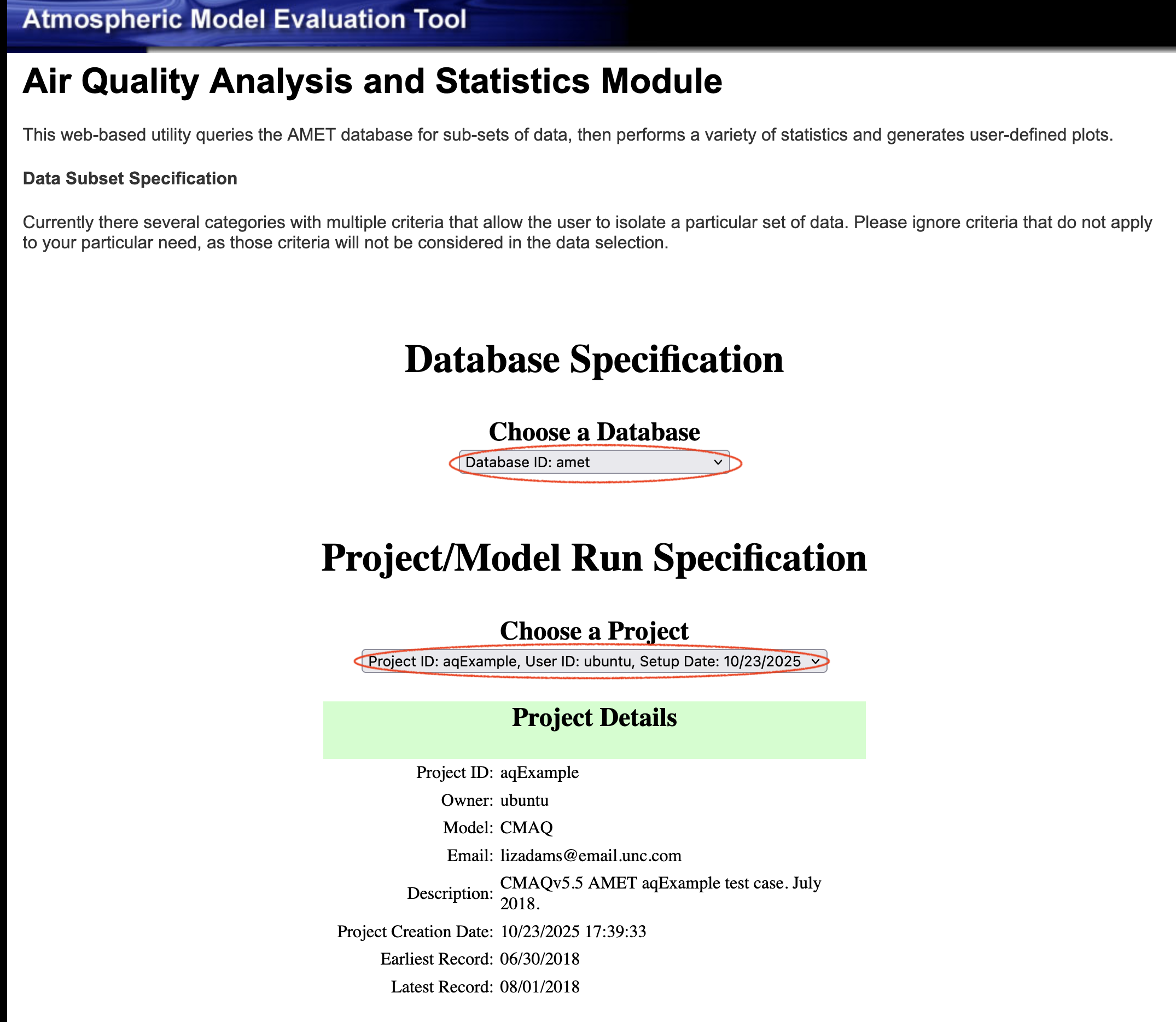
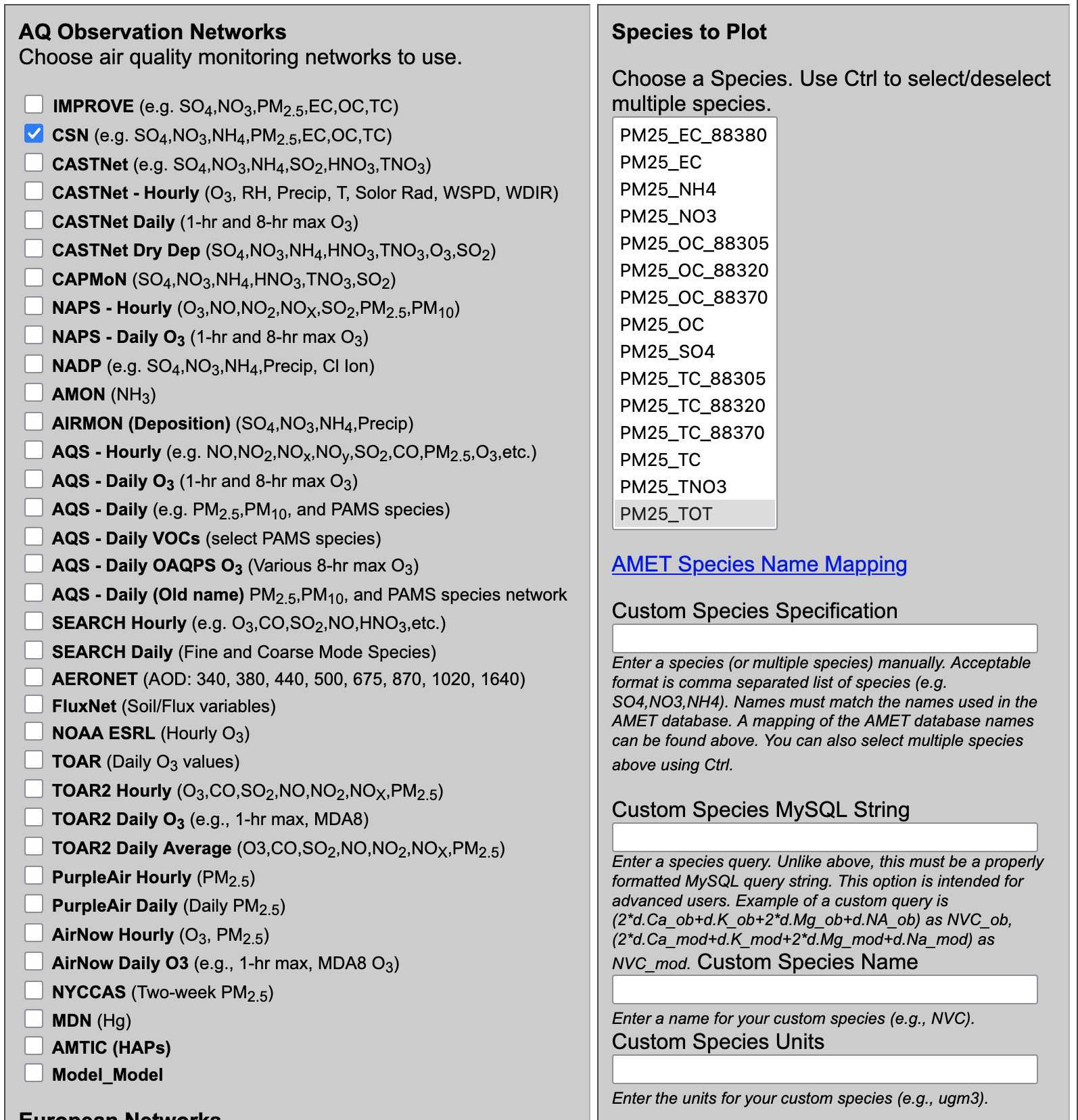
Verify you see the website and that it looks similar to the image below.

Use the website to select the database, project, observation network, variables to plot, and plotting programs.

Note, errors may occur when you make incompatible selections on the AMET Website, see a list of typical error types below.

Click on the arrow to display the list the available programs for creating different types of plots.

7.4. Programs to create plots (74)

Scatter Plots (14) | Click to expand!

Name of R Script | Select Program
1. AQ_Scatterplot.R | Multiple Networks Model/Ob Scatterplot (select stats only)
2. AQ_Scatterplot_ggplot.R | GGPlot Scatterplot (multi network, single run)
3. AQ_Scatterplot_plotly.R | Interactive Multiple Network Scatterplot
4. AQ_Scatterplot_multisim_plotly.R | Interactive Multiple Simulation Scatterplot
5. AQ_Scatterplot_single.R | Single Network Model/Ob Scatterplot (includes all stats)
6. AQ_Scatterplot_density.R | Density Scatterplot (single run, single network)
7. AQ_Scatterplot_density_ggplot.R | GGPlot Density Scatterplot (single run, single network)
8. AQ_Scatterplot_mtom.R | Model/Model Scatterplot (multiple networks)
9. AQ_Scatterplot_mtom_density_ggplot.R | Model/Model Density Scatterplot (single network)
10. AQ_Scatterplot_percentiles.R | Scatterplot of Percentiles (single network, single run)
11. AQ_Scatterplot_skill.R | Ozone Skill Scatterplot (single network, mult runs)
12. AQ_Scatterplot_bins.R | Binned MB & RMSE Scatterplots (single net., mult. run)
13. AQ_Scatterplot_bins_plotly.R | Interactive Binned Plot (single net., mult. run)
14. AQ_Scatterplot_multi.R | Multi Simulation Scatter plot (single network, mult runs)

Timeseries Plots (12) | Click to expand!

Name of R Script | Program
1. AQ_Timeseries.R | Time-series Plot (single network, multiple sites averaged)
2. AQ_Timeseries_bysite.R | Individual Site Time-series Plots (single network, multiple sites not average)
3. AQ_Timeseries_dygraph.R | Dygraph Time-series Plot (single network, multiple sites averaged)
4. AQ_Timeseries_plotly.R | Plotly Muli-simulation Timeseries
5. AQ_Timeseries_plotly_bysite.R | Individual Site Plotly Time-series Plots (single network, multiple sites not average)
6. AQ_Timeseries_networks_plotly.R | Plotly Multi-network Timeseries
7. AQ_Timeseries_species_plotly.R | Plotly Multi-species Timeseries
8. AQ_Timeseries_multi_networks.R | Multi-Network Time-series Plot (mult. net., single run)
9. AQ_Timeseries_multi_species.R | Multi-Species Time-series Plot (mult. species, single run)
10. AQ_Timeseries_MtoM.R | Model-to-Model Time-series Plot (single net., multi run)
11. AQ_Monthly_Stat_Plot.R | Year-long Monthly Statistics Plot (single network)
12. AQ_Monthly_Stat_Plot_plotly.R | Interactive Year-long Monthly Statistics Plot (single network)

Spatial Plots (14) | Click to expand!

Name of R Script | Program
1. AQ_Stats_Plots.R | Species Statistics and Spatial Plots (multi networks)
2. AQ_Stats_Plots_leaflet.R | Interactive Species Statistics and Spatial Plots (single plot)
3. AQ_Stats_Plots_leaflet_network.R | Interactive Species Statistics and Spatial Plots (multiple plots)
4. AQ_Plot_Spatial.R | Spatial Plot (multi networks)
5. AQ_Plot_Spatial_leaflet.R | Interactive Spatial Plot
6. AQ_Plot_Spatial_leaflet_network.R | Interactive Spatial Plot (multiple plots)
7. AQ_Plot_Spatial_Species_Diff_leaflet.R | Interactive Species Diff Spatial Plot (multi networks,multi species)
8. AQ_Plot_Spatial_MtoM.R | Model/Model Diff Spatial Plot (multi network, multi run)
9. AQ_Plot_Spatial_MtoM_leaflet.R | Interactive Model/Model Diff Spatial Plot (multi network, multi run)
10. AQ_Plot_Spatial_MtoM_Species.R | Model/Model Species Diff Spatial Plot (multi network, multi run)
11. AQ_Plot_Spatial_Diff.R | Spatial Plot of Bias/Error Difference (multi network, multi run)
12. AQ_Plot_Spatial_Diff_leaflet.R | Interactive Spatial Plot of Bias/Error Difference (single plot)
13. AQ_Plot_Spatial_Diff_leaflet_network.R | Interactive Spatial Plot of Bias/Error Difference (multiple plots)
14. AQ_Plot_Spatial_Ratio.R | Ratio Spatial Plot to total PM2.5 (multi network, multi run)

Box Plots (7) | Click to expand!

Name of R Script | Program
1. AQ_Boxplot.R | Boxplot (single network, multi run)
2. AQ_Boxplot_ggplot.R | GGPlot Boxplot (single network, multi run)
3. AQ_Boxplot_plotly.R | Plotly Boxplot (single network, multi run)
4. AQ_Boxplot_DofW.R | Day of Week Boxplot (single network, multiple runs)
5. AQ_Boxplot_Hourly.R | Hourly Boxplot (single network, multiple runs)
6. AQ_Boxplot_MDA8.R | 8hr Average Boxplot (single network, hourly data, can be slow)
7. AQ_Boxplot_Roselle.R | Roselle Boxplot (single network, multiple simulations)

Stacked Bar Plots (9) | Click to expand!

Name of R Script | Program
1. AQ_Stacked_Barplot.R | PM2.5 Stacked Bar Plot (CSN or IMPROVE, multi run)
2. AQ_Stacked_Barplot_AE6.R | PM2.5 Stacked Bar Plot AE6 (CSN or IMPROVE, multi run)
3. AQ_Stacked_Barplot_AE6_plotly.R | Interactive Stacked Bar Plot
4. AQ_Stacked_Barplot_AE6_ggplot.R | GGPlot Stacked Bar Plot
5. AQ_Stacked_Barplot_AE6_ts.R | Stacked Bar Plot Time Series
6. AQ_Stacked_Barplot_soil_multi.R | Soil Stacked Bar Plot Multi (CSN and IMPROVE,single run)
7. AQ_Stacked_Barplot_panel.R | Multi-Panel Stacked Bar Plot (full year data required)
8. AQ_Stacked_Barplot_panel_AE6.R | Multi-Panel Stacked Bar Plot AE6 (full year data)
9. AQ_Stacked_Barplot_panel_AE6_multi.R | Multi-Panel, Mulit Run Stacked Bar Plot AE6 (full year data)

Misc Plots (14) | Click to expand!

Name of R Script | Program
1. AQ_Kellyplot.R | Kelly Plot (single species, single network, full year data)
2. AQ_Kellyplot_plotly.R | Plotly Kelly Plot (single species, single network, full year data)
3. AQ_Kellyplot_region.R | Climate Region Kelly Plot (single species, single network, multi sim)
4. AQ_Kellyplot_region_plotly.R | Plolty Climate Region Kelly Plot (single species, single network, multi sim)
5. AQ_Kellyplot_season.R | Seasonal Kelly Plot (single species, single network, multi sim)
6. AQ_Kellyplot_season_plotly.R | Plotly Seasonal Kelly Plot (single species, single network, multi sim)
7. AQ_Stats.R | Species Statistics (multi species, single network)
8. AQ_Raw_Data.R | Create raw data csv file (single network, single simulation)
9. AQ_Soccerplot.R | Soccergoal" plot (multiple networks)
10. AQ_Soccerplot_plotly.R | Plotly "Soccergoal" plot (multiple networks/species)
11. AQ_Bugleplot.R | "Bugle" plot (multiple networks)
12. AQ_Histogram.R | Histogram (single network/species only)
13. AQ_Histogram_plotly.R | Interactive Histogram (single network, single species, multi run)
14. AQ_Temporal_Plots.R | CDF, Q-Q, Taylor Plots (single network, multi run)

Experimental Scripts (4) | Click to expand!

Name of R Script | Program (may not work correctly)
1. AQ_Overlay_File.R | Create PAVE/VERDI Obs Overlay File (hourly/daily data only)
2. AQ_Scatterplot_log.R | Log-Log Model/Ob Scatterplot (multiple networks)
3. AQ_Spectral_Analysis.R | Spectral Analysis (single network, single run, experimental)
4. AQ_Plot_Spatial_Ratio.R | PM Ratio Spatial Plot (multi network, single run)

7.5. Air Quality Observation Networks (48)

Note, not all databases have all observation networks, and observation networks have different observed species.

 select distinct network from aqExample;
+-------------------+
| network           |
+-------------------+
| AQS_Daily         |
| AQS_Daily_O3      |
| AQS_Hourly        |
| CASTNET           |
| CASTNET_Daily     |
| CASTNET_Drydep    |
| CASTNET_Drydep_O3 |
| CASTNET_Hourly    |
| CSN               |
| IMPROVE           |
| NADP              |
| NAPS              |
| NAPS_Daily_O3     |
+-------------------+

select distinct network from CMAQv532_12US1_2002;
+---------------+
| network       |
+---------------+
| AQS_Daily     |
| AQS_Daily_O3  |
| AQS_Hourly    |
| CASTNET_Daily |
+---------------+

AQ Observation Networks (35) | Click to expand!

Name of US Air Quality Monitoring Network
1. IMPROVE (e.g. SO4,NO3,PM2.5,EC,OC,TC)
2. CSN (e.g. SO4,NO3,NH4,PM2.5,EC,OC,TC)
3. CASTNet (e.g. SO4,NO3,NH4,SO2,HNO3,TNO3)
4. CASTNet - Hourly (O3, RH, Precip, T, Solor Rad, WSPD, WDIR)
5. CASTNet Daily (1-hr and 8-hr max O3)
6. CASTNet Dry Dep (SO4,NO3,NH4,HNO3,TNO3,O3,SO2)
7. CAPMoN (SO4,NO3,NH4,HNO3,TNO3,SO2)
8. NAPS - Hourly (O3,NO,NO2,NOX,SO2,PM2.5,PM10)
9. NAPS - Daily O3 (1-hr and 8-hr max O3)
10. NADP (e.g. SO4,NO3,NH4,Precip, Cl Ion)
11. AMON (NH3)
12. AIRMON (Deposition) (SO4,NO3,NH4,Precip)
13. AQS - Hourly (e.g. NO,NO2,NOx,NOy,SO2,CO,PM2.5,O3,etc.)
14. AQS - Daily O3 (1-hr and 8-hr max O3)
15. AQS - Daily (e.g. PM2.5,PM10, and PAMS species)
16. AQS - Daily VOCs (select PAMS species)
17. AQS - Daily OAQPS O3 (Various 8-hr max O3)
18. AQS - Daily (Old name) PM2.5,PM10, and PAMS species network
19. SEARCH Hourly (e.g. O3,CO,SO2,NO,HNO3,etc.)
20. SEARCH Daily (Fine and Coarse Mode Species)
21. AERONET (AOD: 340, 380, 440, 500, 675, 870, 1020, 1640)
22. FluxNet (Soil/Flux variables)
23. NOAA ESRL (Hourly O3)
24. TOAR (Daily O3 values)
25. TOAR2 Hourly (O3,CO,SO2,NO,NO2,NOX,PM2.5)
26. TOAR2 Daily O3 (e.g., 1-hr max, MDA8)
27. TOAR2 Daily Average (O3,CO,SO2,NO,NO2,NOX,PM2.5)
28. PurpleAir Hourly (PM2.5)
29. PurpleAir Daily (Daily PM2.5)
30. AirNow Hourly (O3, PM2.5)
31. AirNow Daily O3 (e.g., 1-hr max, MDA8 O3)
32. NYCCAS (Two-week PM2.5)
33. MDN (Hg)
34. AMTIC (HAPs)
35. Model_Model

European Networks (10) | click to expand!

Name of European Network
1. ADMN (SO4,NO3,NH4,Precip, Na Ion, Cl Ion)
2. AGANET (HCl, NO2, NOY, SOX, HNO3, SO2, Cl, Na)
3. AirBase_Hourly (NO, NO2, NOX, SO2, CO, PM2.5, PM10, O3)
4. AirBase_Daily (NO, NO2, NOX, SO2, CO, PM2.5, PM10, O3)
5. AURN_Hourly (NO, NO2, NOX, SO2, CO, PM2.5, PM10, O3)
6. AURN_Daily (NO, NO2, NOX, SO2, CO, PM2.5, PM10, O3)
7. EMEP - Hourly (NO, NO2, NOX, SO2, CO, PM2.5, PM10, O3)
8. EMEP - Daily (SO4, NO3, NH44, trace metals, PM2.5, PM10, O3)
9. EMEP - Daily O3 (1-rh and 8-hr max O3)
10. EMEP - Dep (SO4, NO3, NH44, Cl, Na, trace metals)

Campaigns (3) | Click to expand!

Name of Campaign
1. CALNEX
2. SOAS
3. Special

Additional details about observation networks:

Earth Engine Applet for Visualizing NADP Total Deposition (TDep) of Total Sulfur and Nitrogen Deposition

AirData Air Quality Monitors

Map of AQS

About AQS Data

CASTNET sites provide air quality data in rural locations

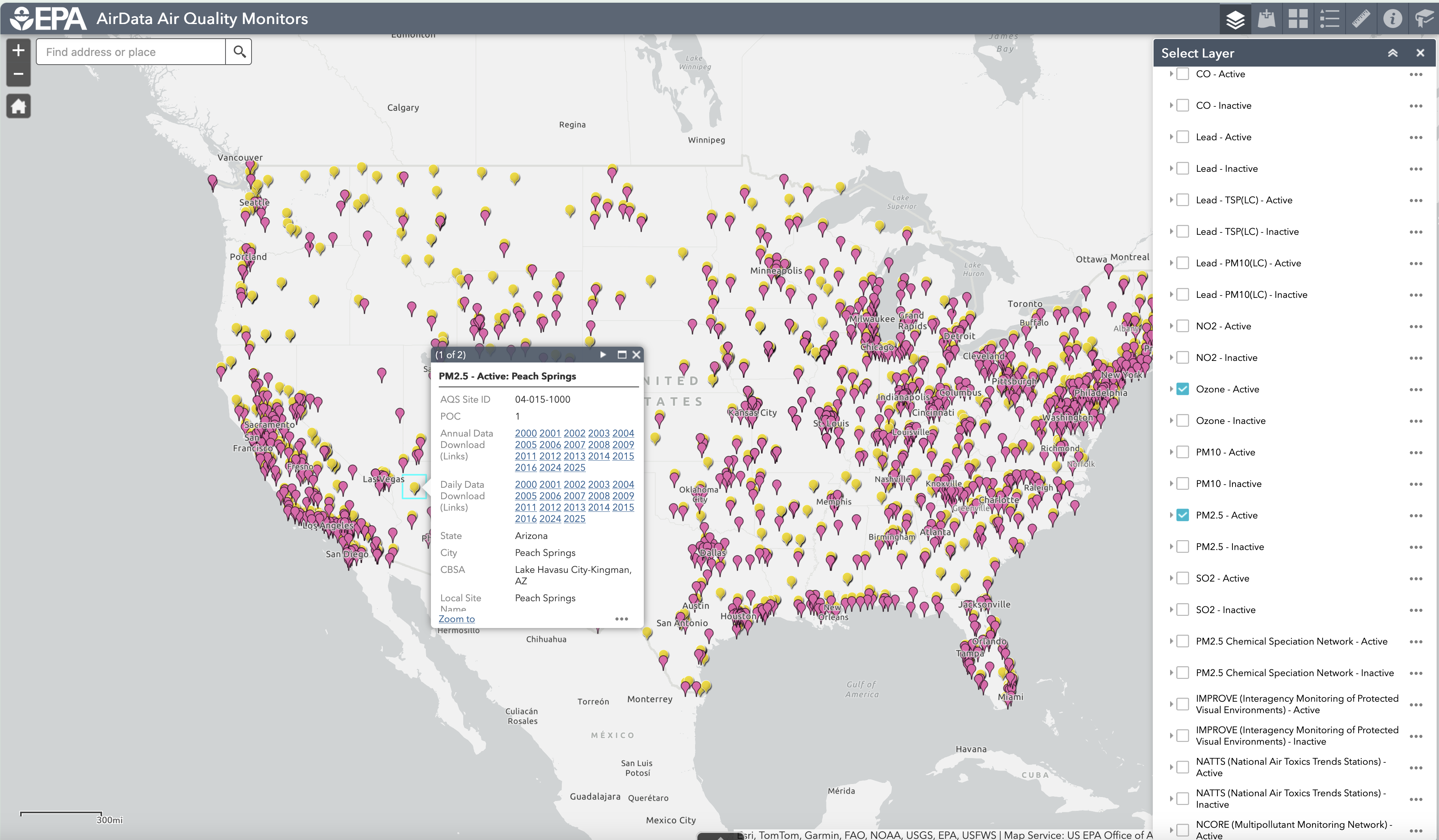
Interactive Map of Air Quality Monitors

US EPA Nonattainment Areas and Designations - PM2.5 Daily (24-hour) (2006 NAAQS)

PM2.5 Speciation Data 2021-2023, US EPA, OAR, OAQPS

Chemical Speciation Network (CSN) Monitor Locations and Information

Ambient Air Monitoring Networks

Interagency Monitoring of Protected Visual Environments

National Parks in the History of Science: Visibility (Video)

7.6. Air Quality and Met Species (172)

Note, to get started with creating plots using AMET, it is best to use a subset of the species listed under Species to Plot. The examples in this documentation use one or more of the following five criteria air pollutants: particulate matter (PM25_TOT, PM10_TOT), ground-level ozone (O3, O3_8hrmax, O3_1hrmax), sulfur dioxide (SO2), carbon monoxide (CO) and nitrogen dioxide (NO2, NOX, NOY), along with NO3 (Nitrate) and NH4 ammonium which are key component of secondary inorganic fine particulate matter, and VOCs including Ethylene, Isoprene, Tolulene that react with NOX to form Ozone.

List of AQ Species available for EQUATES (40) | Click to expand!

Species available for EQUATES
1. SO4
2. NO3
3. NH4
4. EC
5. OC
6. TC
7. other, PMOther
8. ncom
9. Cl, Cl Ion
10. Na, Na Ion
11. PM_TOT, PM2.5 Mass(I+J)
12. PM_FRM, PM2.5 FRM Equiv.(I+J)
13. PM25_SO4, PM2.5 SO4
14. PM25_NO3, PM_2.5 NO3
15. PM25_NH4, PM_2.5 NH4
16. PM25_TOT, PM_2.5 Total Mass
17. PM25_FRM, PM_2.5 FRM Equiv.
18. PM25_EC, PM_2.5 EC
19. PM25_OC, PM_2.5 OC
20. PM25_TC, PM_2.5 TC
21. PM25_Cl, PM_2.5 Cl Ion
22. PM25_Na, PM_2.5 Na Ion
23. PMC_SO4, PM_Coarse SO4
24. PMC_NO3, PM_Coarse NO3
25. PMC_NH4, PM_Coarse NH4
26. PMC_TOT, PM_Coarse Total Mass
27. PMC_Cl, PM_Coarse Cl Ion
28. PMC_Na, PM_Coarse Na Ion
29. PM10, PM10 Mass
30. Na, Sodium(Na)
31. Cl, Chlorine(Cl)
32. Fe, Iron(Fe)
33. Al, Aluminium(Al)
34. Si, Silicon(Si)
35. Ti, Titanium(Ti)
36. Ca, Calcium(Ca)
37. Mg, Magnesium(Mg)
38. K, Potassium(K)
39. Mn, Mangenese(Mn)
40. soil, Soil(IMPROVE Eqn.)

Subset of variables available for aqExample (126) | Click to expand!

Note, not all species are available at all observation networks. Example: PAMS Network has select VOCs, NO and NO2. Species available for PAMS Observation Network

Subset of Gas phase variables (24)
1. O3, Ozone (hourly or daily)
2. O3_1hrmax, Ozone 1-hrmax(daily)
3. O3_8hrmax, Ozone 8-hrmax(daily)
4. O3_1hrmax_9cell, Ozone 1-hrmax 9-cell avg(daily)
5. O3_8hrmax_9cell, Ozone 8-hrmax 9-cell avg(daily)
6. O3_1hrmax_time, Ozone 1-hrmax hour(daily)
7. SO2
8. NH3
9. HNO3
10. TNO3, TNO3(NO3+HNO3)
11. CO
12. NO
13. NO2
14. NOX
15. NOY
16. H2O2
17. HOx
18. Acetaldehyde
19. Formaldehyde
20. Benzene
21. Ethane
22. Ethylene
23. Isoprene
24. Toluene

Subset of Particles(40)
1. SO4
2. NO3
3. NH4
4. EC
5. OC
6. TC
7. other, PMOther
8. ncom
9. Cl, Cl Ion
10. Na, Na Ion
11. PM_TOT, PM2.5 Mass(I+J)
12. PM_FRM, PM2.5 FRM Equiv.(I+J)
13. PM25_SO4, PM2.5 SO4
14. PM25_NO3, PM_2.5 NO3
15. PM25_NH4, PM_2.5 NH4
16. PM25_TOT, PM_2.5 Total Mass
17. PM25_FRM, PM_2.5 FRM Equiv.
18. PM25_EC, PM_2.5 EC
19. PM25_OC, PM_2.5 OC
20. PM25_TC, PM_2.5 TC
21. PM25_Cl, PM_2.5 Cl Ion
22. PM25_Na, PM_2.5 Na Ion
23. PMC_SO4, PM_Coarse SO4
24. PMC_NO3, PM_Coarse NO3
25. PMC_NH4, PM_Coarse NH4
26. PMC_TOT, PM_Coarse Total Mass
27. PMC_Cl, PM_Coarse Cl Ion
28. PMC_Na, PM_Coarse Na Ion
29. PM10, PM10 Mass
30. Na, Sodium(Na)
31. Cl, Chlorine(Cl)
32. Fe, Iron(Fe)
33. Al, Aluminium(Al)
34. Si, Silicon(Si)
35. Ti, Titanium(Ti)
36. Ca, Calcium(Ca)
37. Mg, Magnesium(Mg)
38. K, Potassium(K)
39. Mn, Mangenese(Mn)
40. soil, Soil(IMPROVE Eqn.)

Subset of Wet/Dry Deposition Species (25)
1. SO4_dep, SO4(wetdep)
2. SO4_conc, SO4(wetconc)
3. NO3_dep, NO3(wetdep)
4. NO3_conc, NO3(wetconc)
5. NH4_dep, NH4(wetdep)
6. NH4_conc, NH4(wetconc)
7. Cl_dep, Cl Ion(wetdep)
8. Cl_conc, Cl Ion(wetconc)
9. CA_dep, Ca(wetdep)
10. CA_conc, Ca(wetconc)
11. MG_dep, Mg(wetdep)
12. MG_conc, Mg(wetconc)
13. K_dep, K(wetdep)
14. K_conc, K(wetconc)
15. NA_dep, Na(wetdep)
16. NA_conc, Na(wetconc)
17. HGconc, Hg(wetconc)
18. HGdep, Hg(wetdep)
19. SO4_ddep, SO4(drydep)
20. NO3_ddep, NO3(drydep)
21. NH4_ddep, NH4(drydep)
22. HNO3_ddep, HNO3(drydep)
23. TNO3_ddep, TNO3(drydep)
24. O3_ddep, O3(drydep)
25. SO2_ddep, SO2(drydep)

Subset of Toxics (37)
1. Acrolein
2. Acrylonitrile
3. Acetaldehyde
4. Benzene
5. BR2_C2_12
6. Butadiene, 13Butadiene13
7. Cadmium_PM10
8. Cadmium_PM25
9. Carbontet
10. Chromium_PM10
11. Chromium_PM2
12. CHCL3
13. CL_ETHE
14. CL2
15. CL2_C2_12
16. CL2_ME
17. CL3_ETHE
18. CL4_ETHE
19. CL4_Ethane1122
20. CR_III_PM10
21. CR_III_PM25
22. CR_VI_PM10
23. CR_VI_PM25
24. Dichlorobenzene
25. Formaldehyde
26. Lead_PM10
27. Lead_PM25
28. Manganese_PM10
29. Manganese_PM25
30. MEOH
31. MXYL
32. Nickel_PM10
33. Nickel_PM25
34. OXYL
35. Propdichloride
36. PXYL
37. Toluene

Metorological Species for metExample (6) | Click to Expand!

Metorological Species (6)
1. T(2m), 2 meter Temperature
2. Hourly Precipitation
3. Water Vapor Mixing Ratio
4. Wind Speed
5. Solar Radiation
6. Surface Pressure

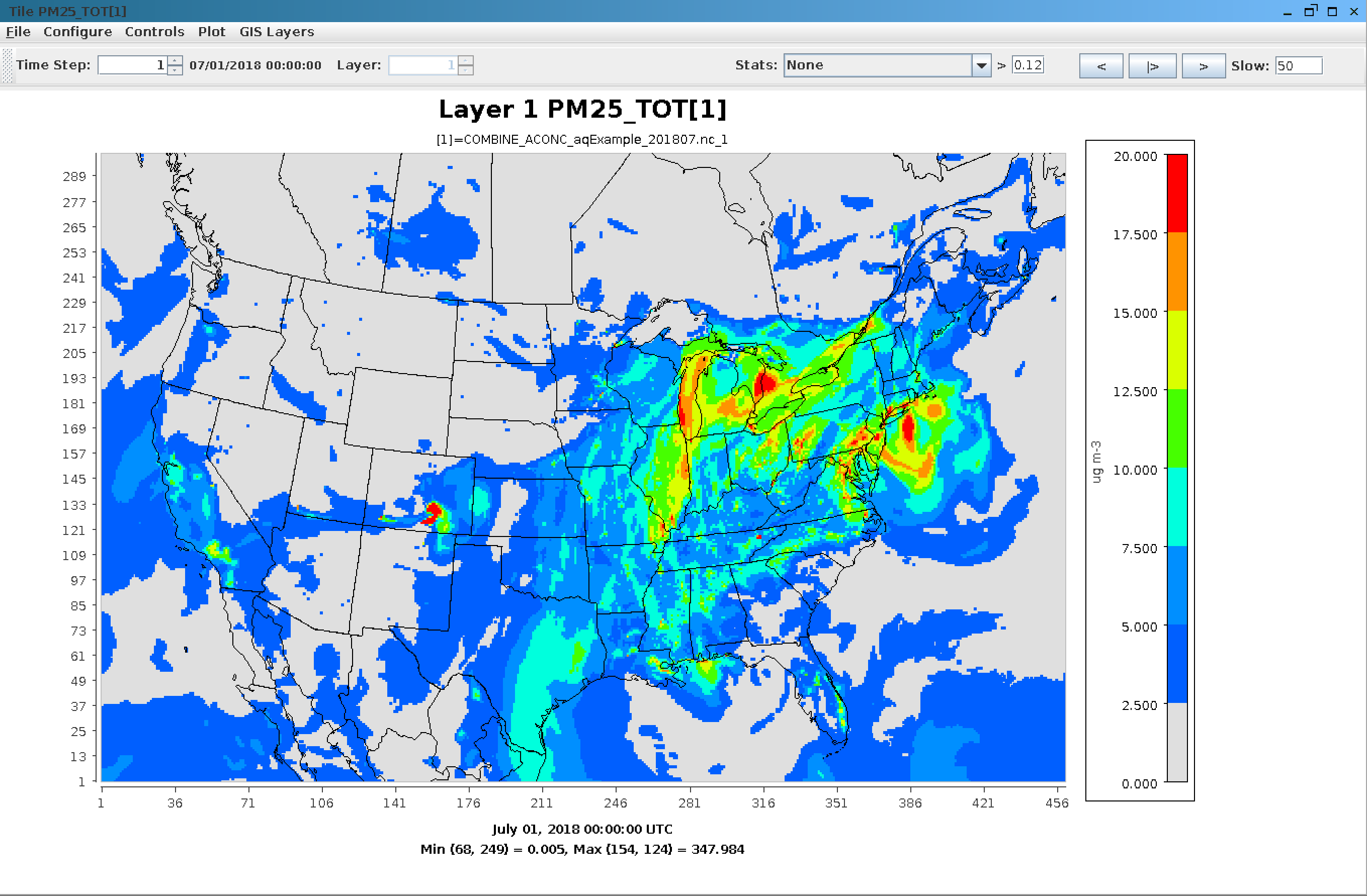
VERDI Plot of PM25_TOT in COMBINE_ACONC_aqExample_201807.nc

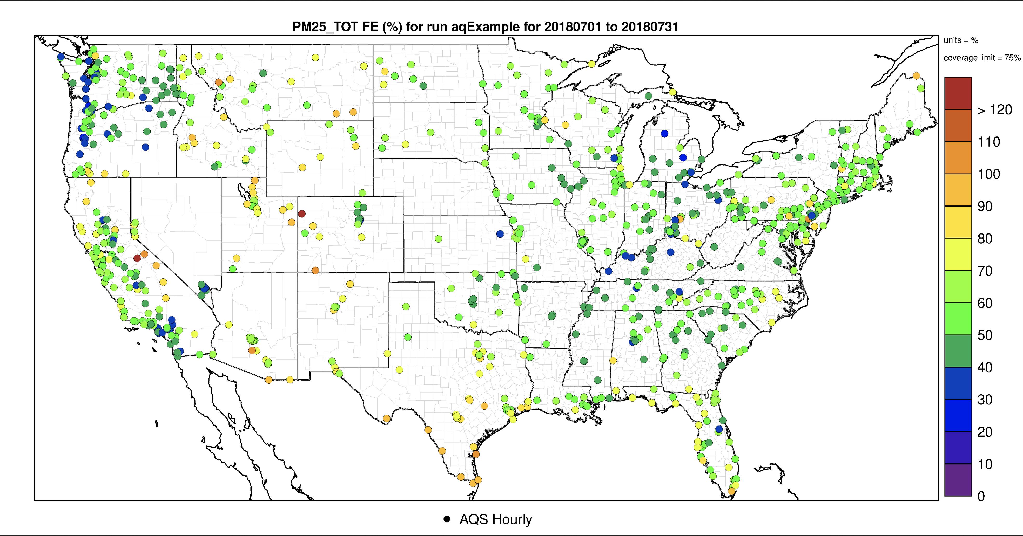
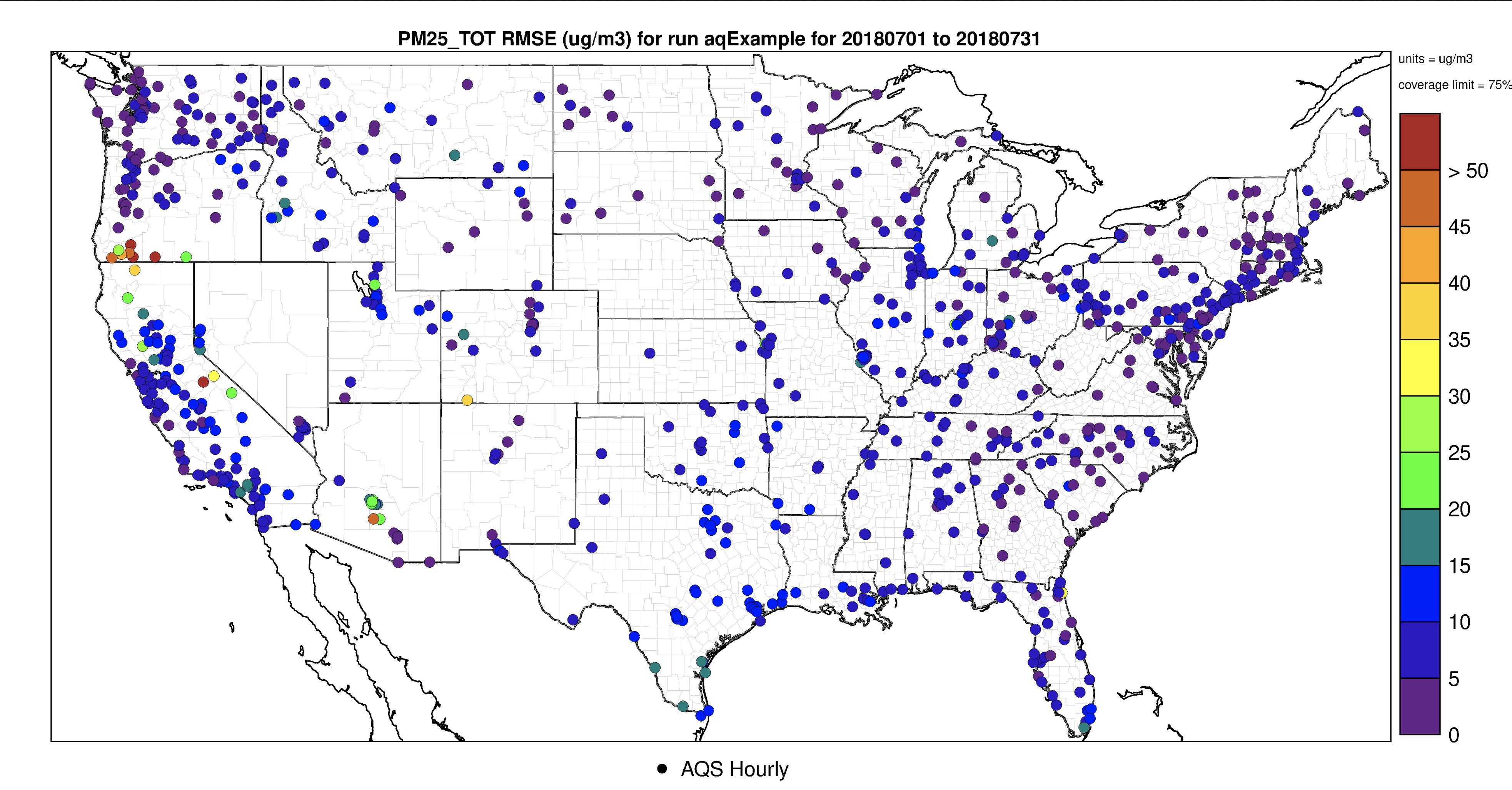
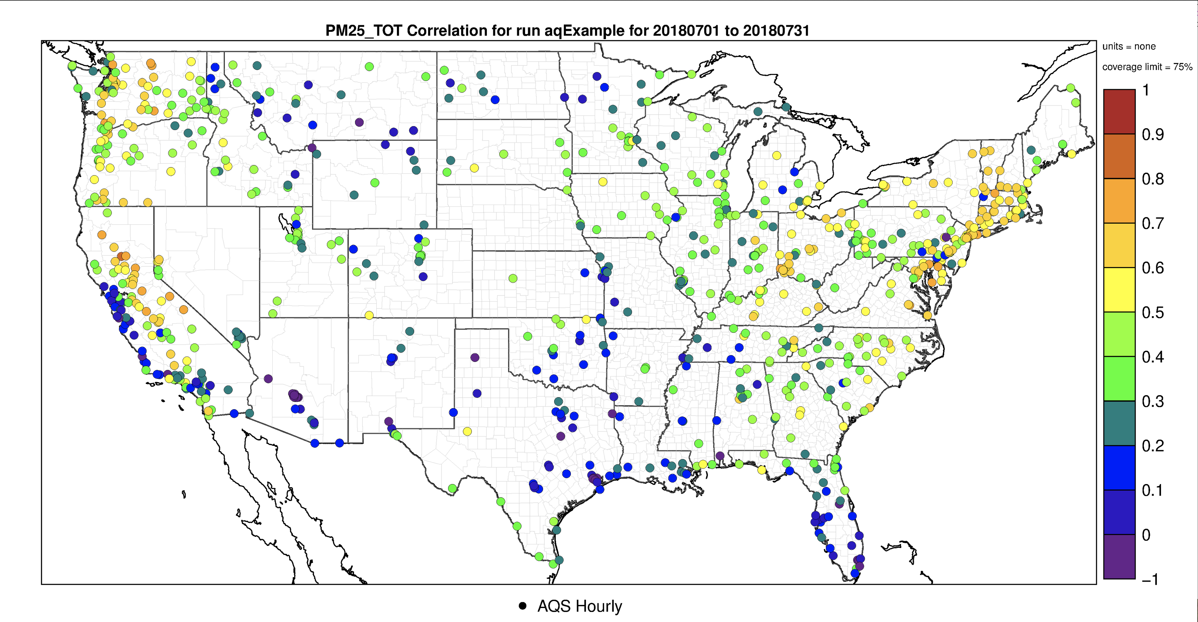
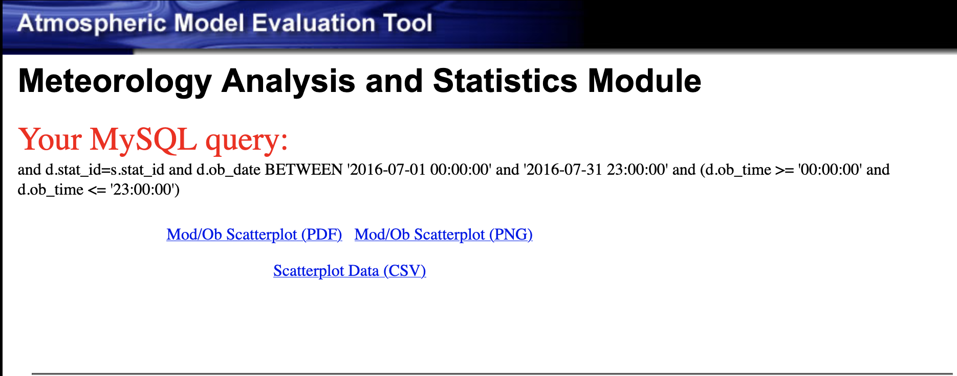
7.7. Method used to create plots

The following is an example of how selections and actions on the website result in the creation of plots.

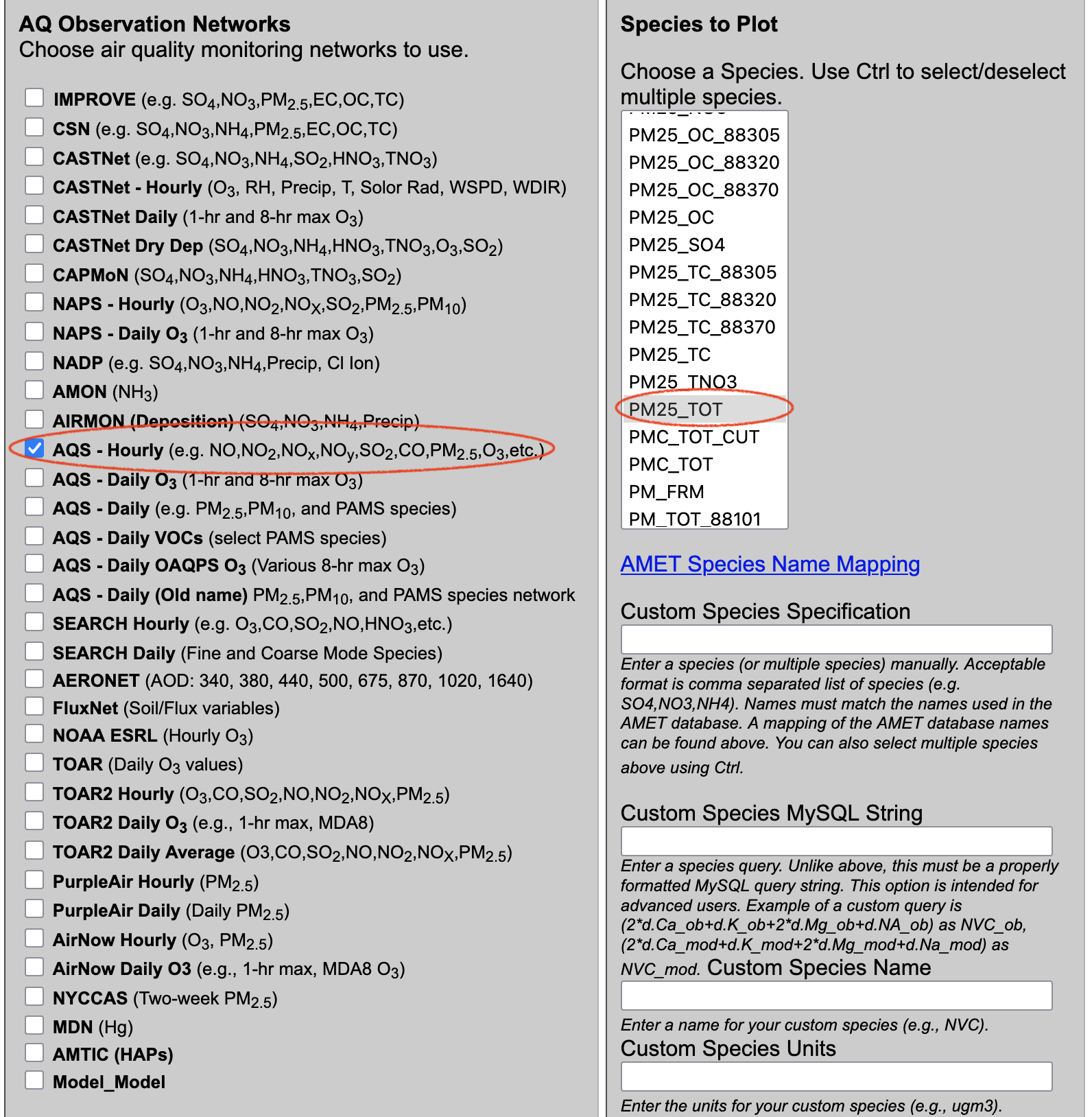
Make the following Website selections and then select Run Program

Choose database: amet
Choose project: aqExample
Choose AQ Network: AQS - Hourly  (e.g. NO,NO2,NOx,NOy,SO2,CO,PM2.5,O3,etc.)
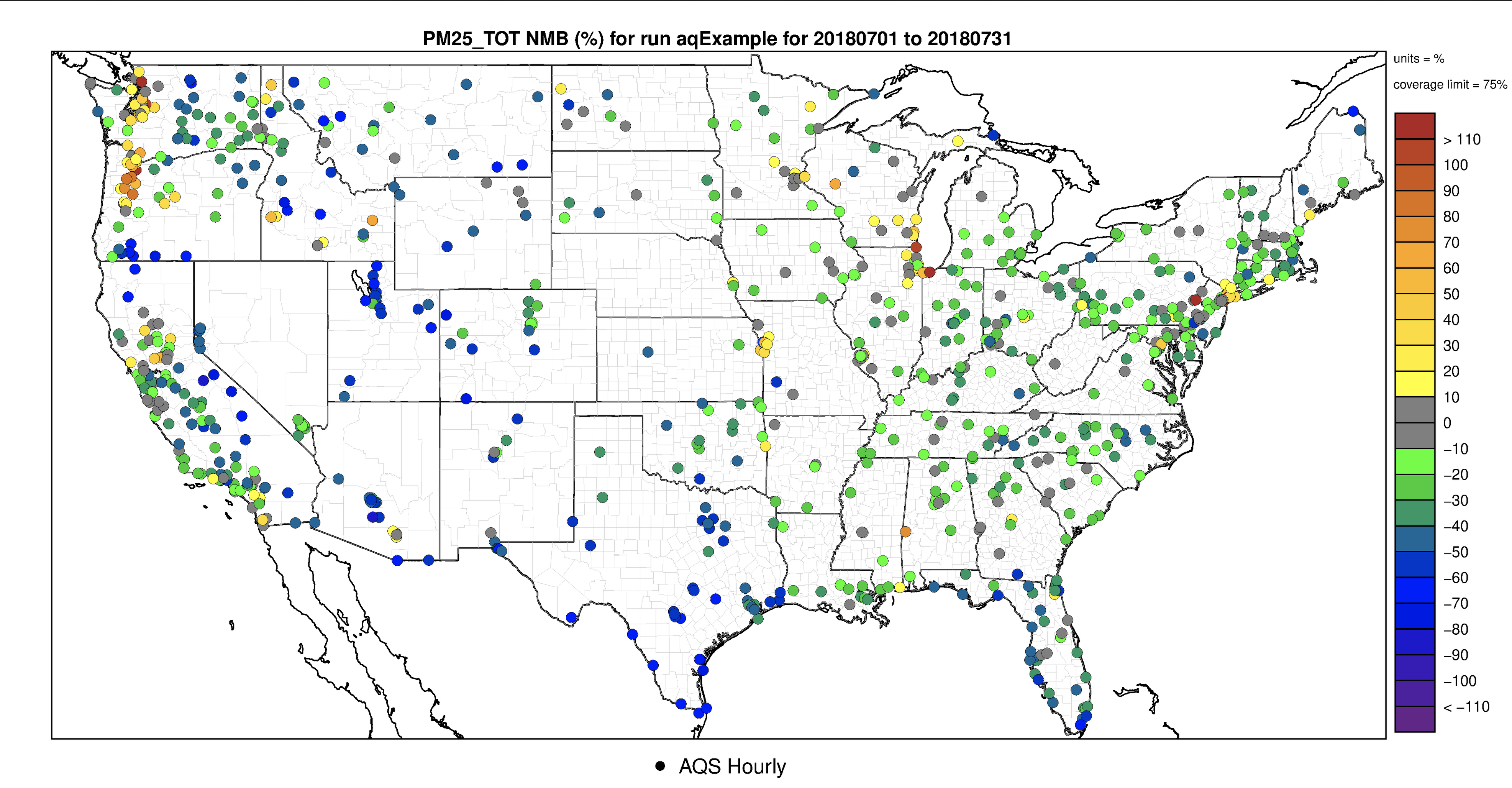
Choose species: PM25_TOT
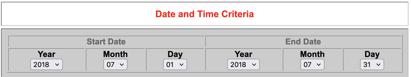
Choose Date/Time Range: 07-01-2018 to 07-31-2018
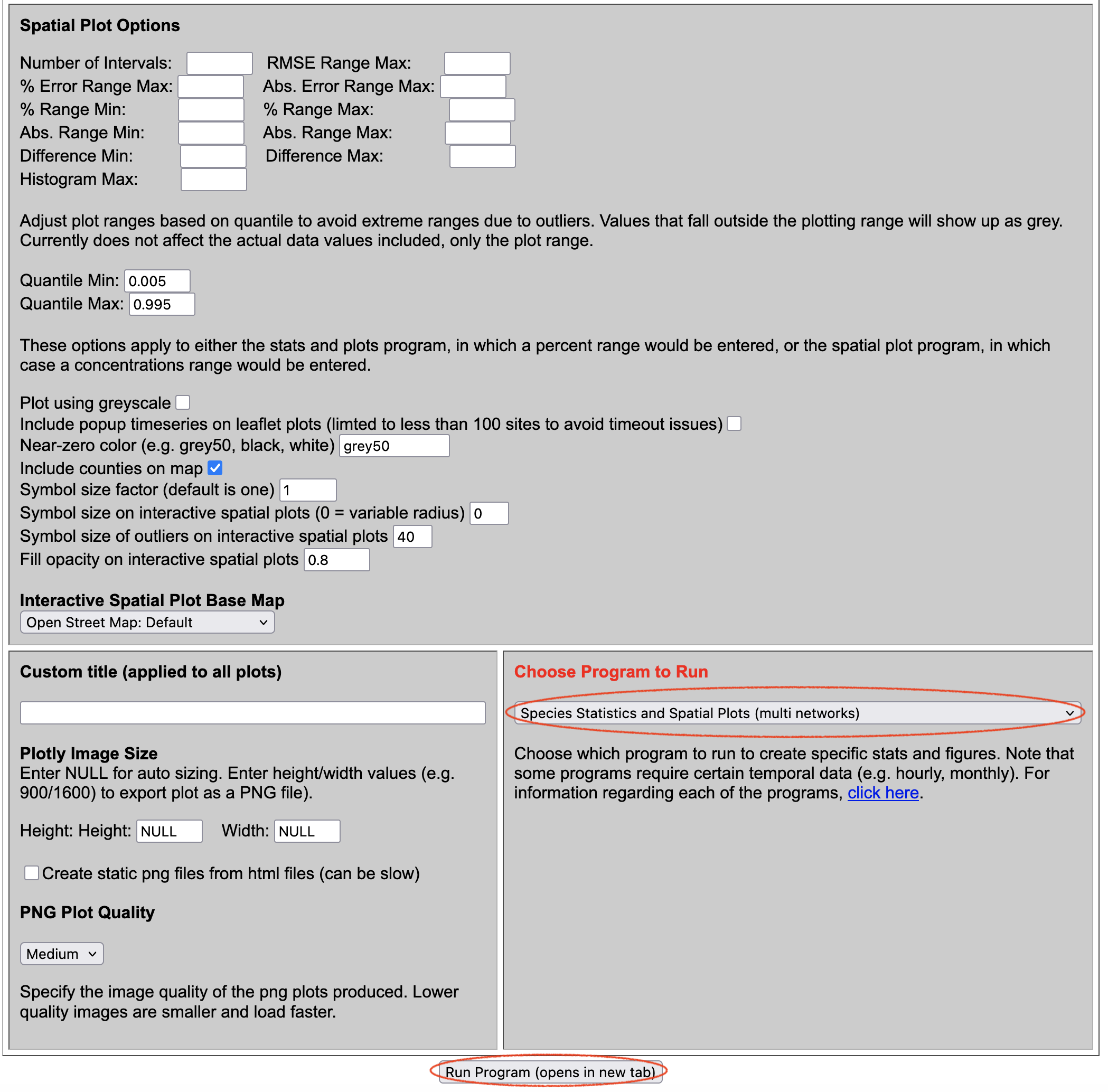
Choose Program: Species Statistics and Spatial Plots (multi networks)

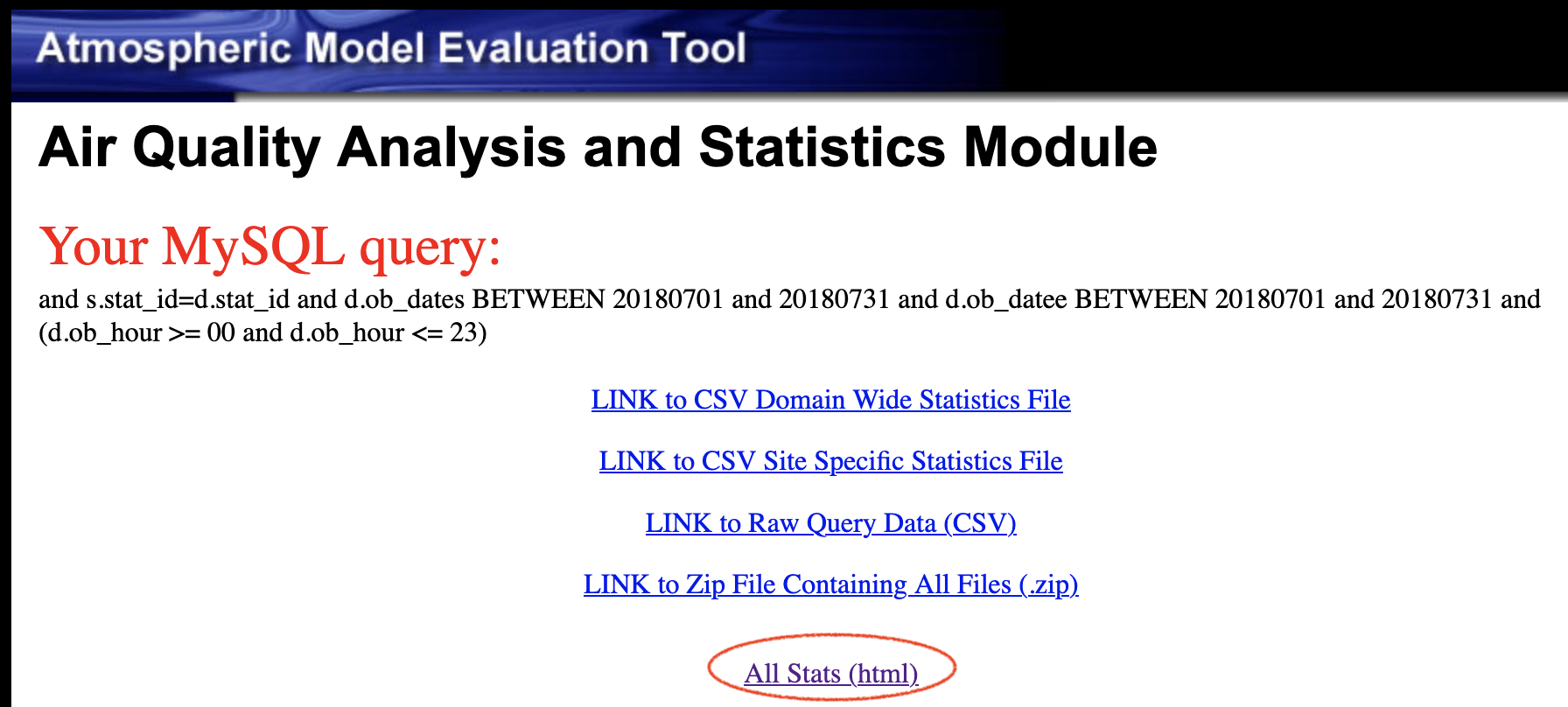
Input selections made on the website (querygen_aq.php or querygen_met.php) are saved as inputs to the run_info.r file under the /var/www/html/cache directory.

The program selection is saved to the run_script.csh, and the run_info.r file is referenced in that run script using the AMETRINPUT environment variable.

Example run script for the program Species Statistics and Spatial Plots, the R program for this plot is named AQ_Stats_Plots.R:

#!/bin/csh -f
cd /var/www/html/cache 
setenv PATH /usr/bin 
setenv R_LIBS /usr/local/lib/R/site-library
setenv AMETBASE /home/ubuntu/AMET_v16
setenv AMETRINPUT /var/www/html/cache/run_info.r
setenv AMET_OUT /var/www/html/cache
setenv MYSQL_CONFIG /var/www/html/amet-config.R
setenv HOME /var/www/html/cache
R CMD BATCH --no-save --verbose /home/ubuntu/AMET_v16/R_analysis_code/AQ_Stats_Plots.R web_query.txt

This is the contents of run_info.r related to the above selections, note: this is not the full file.

### Database Name ###
dbase<-"amet"

### Project ID Name 1 ###
run_name1<-"aqExample"

### Array of Observation Network Flags ###
#inc_networks<-
inc_aqs_hourly<-"y"

### Species ###
species_in<-"PM25_TOT"

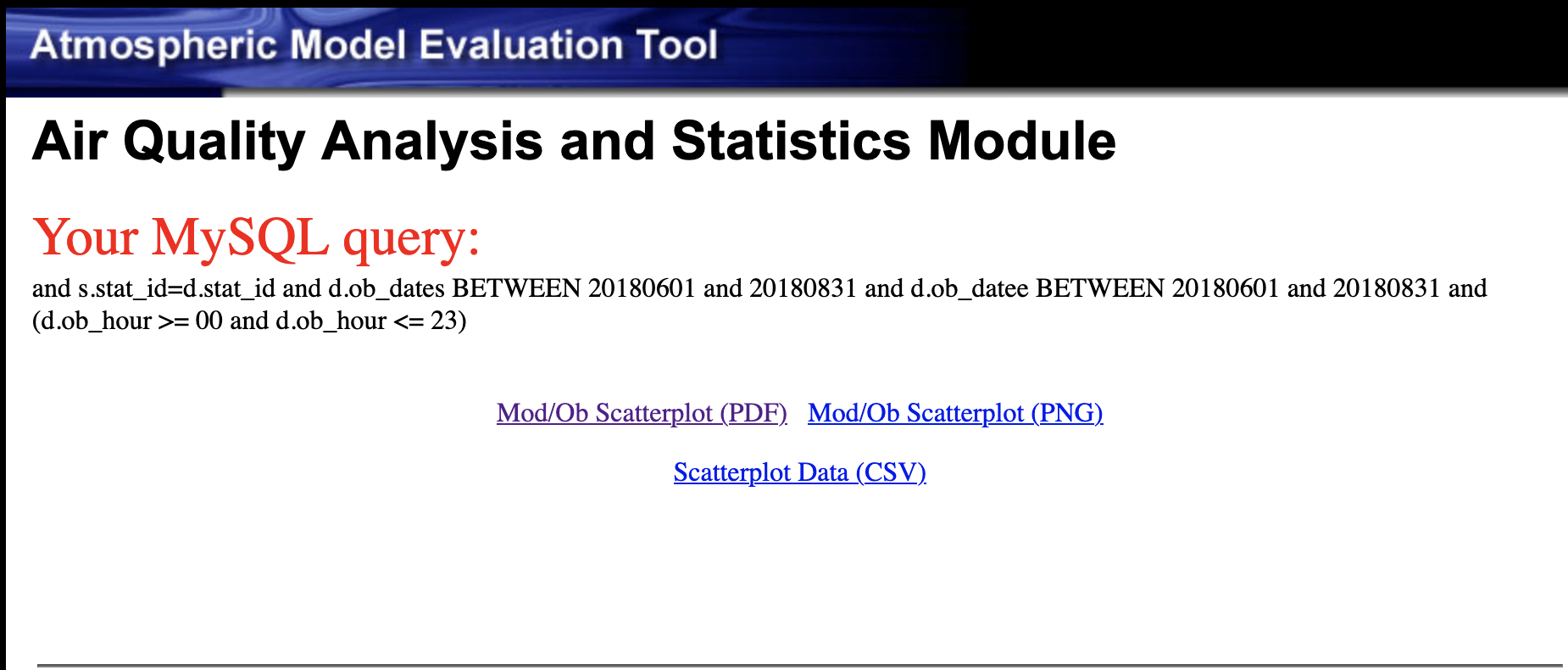
#### Main Database Query String ###
query<-" and s.stat_id=d.stat_id and d.ob_dates BETWEEN 20180701 and 20180731 and d.ob_datee BETWEEN 20180701 and 20180731 and (d.ob_hour >= 00 and d.ob_hour <= 23) "

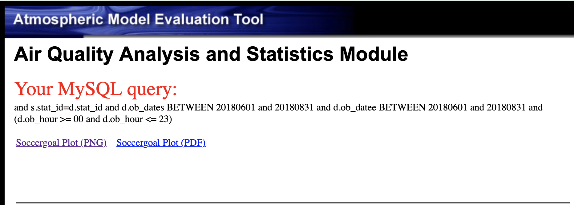
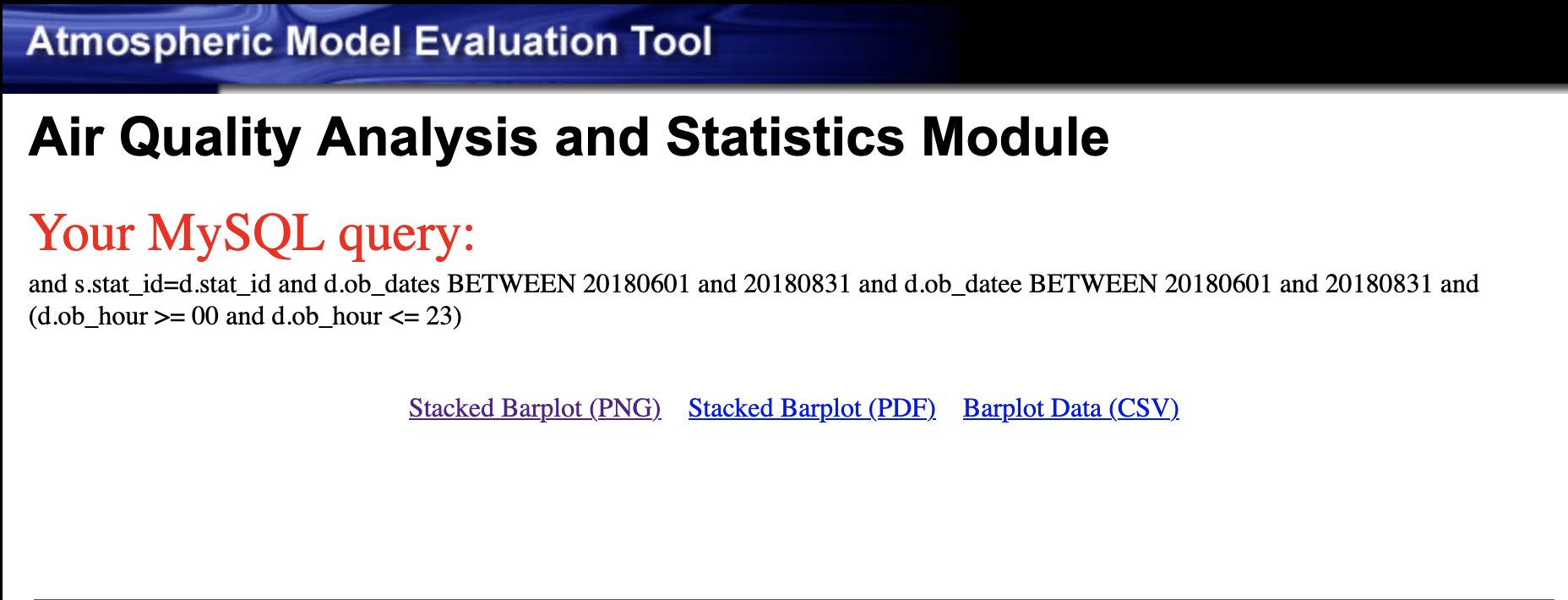
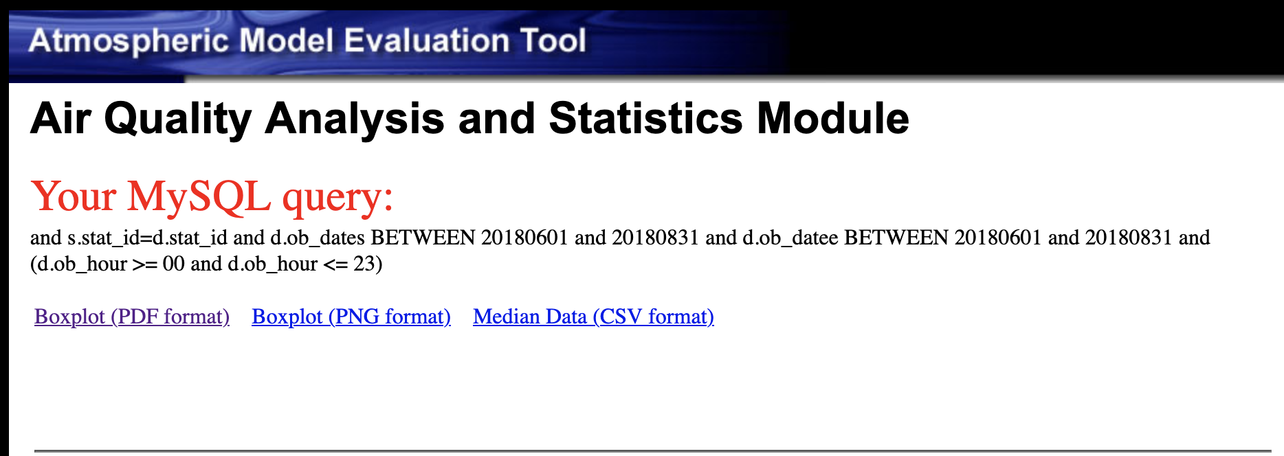
The run_script.csh is run on the Virtual Machine and links to the resulting plots are displayed in another tab on the browser, or an error message is displayed with a link to the web_query.txt.

7.8. Example plots using the aqExample database

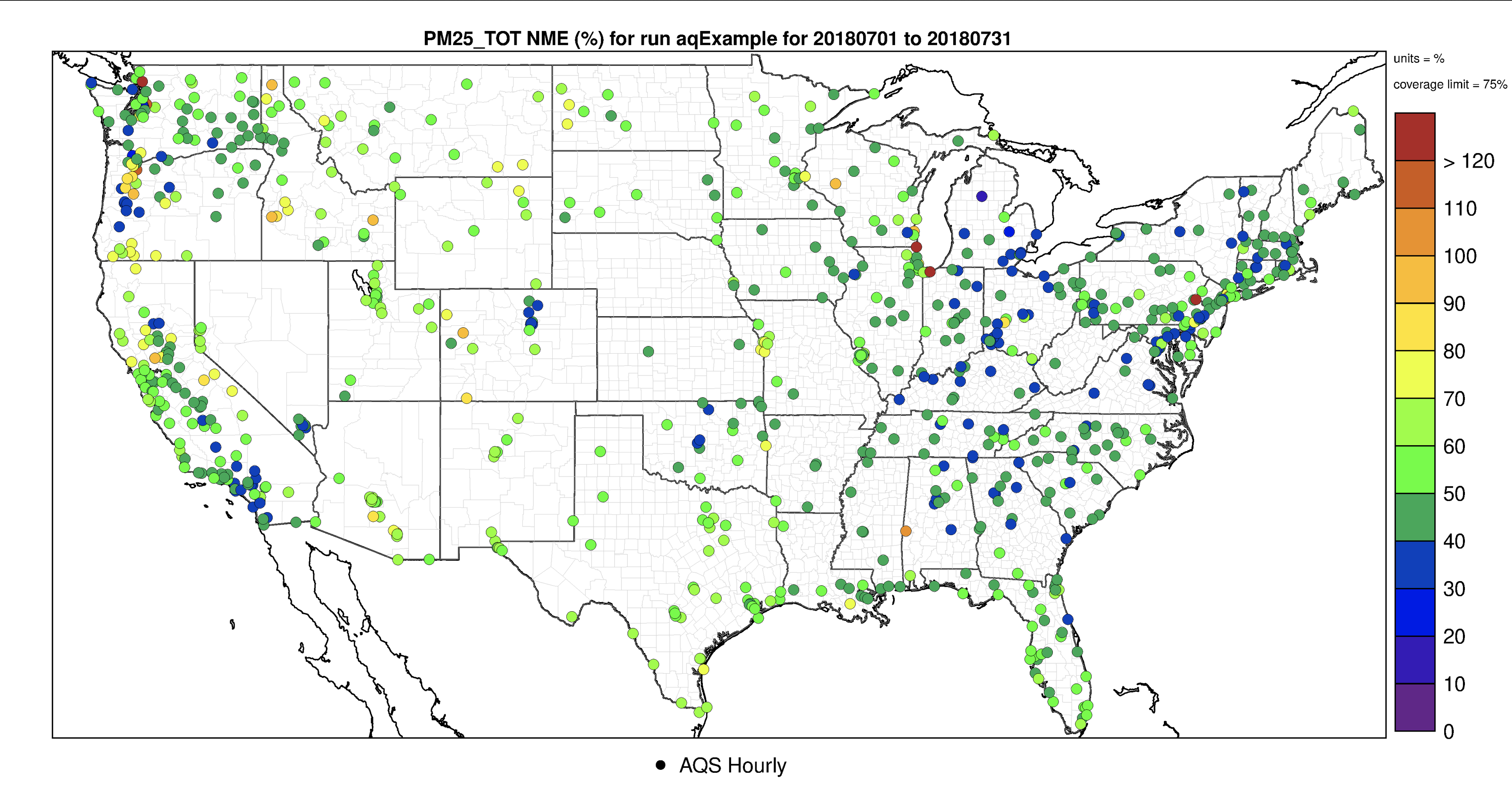
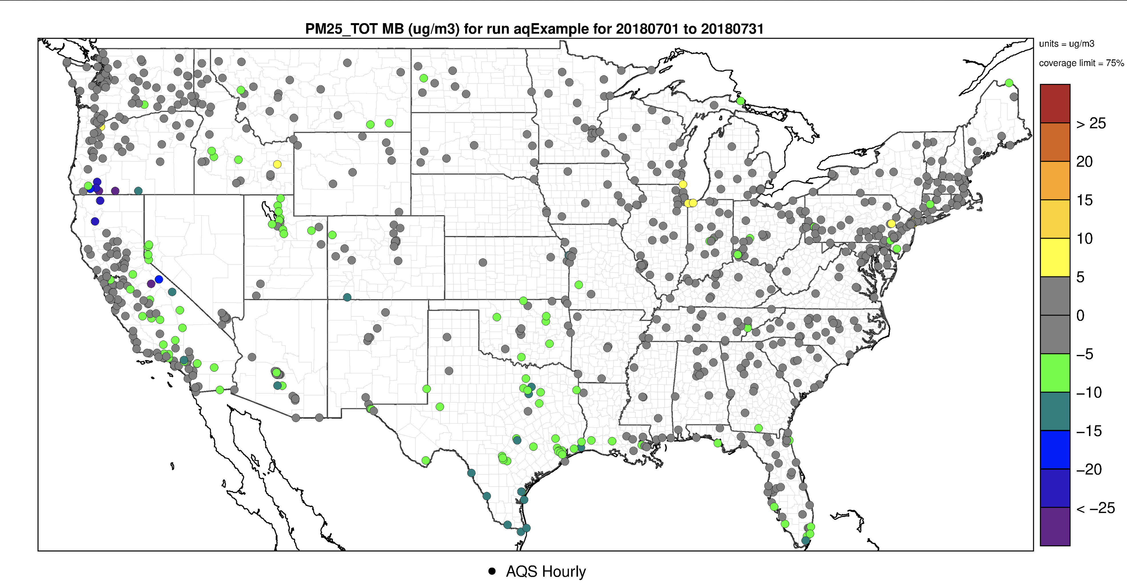
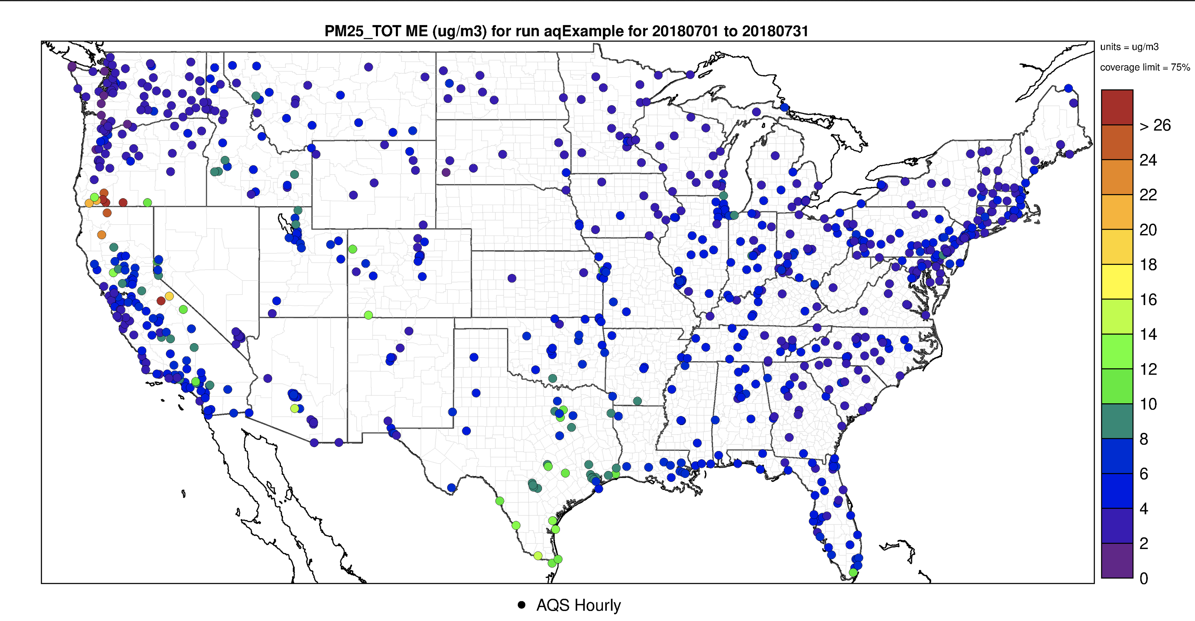
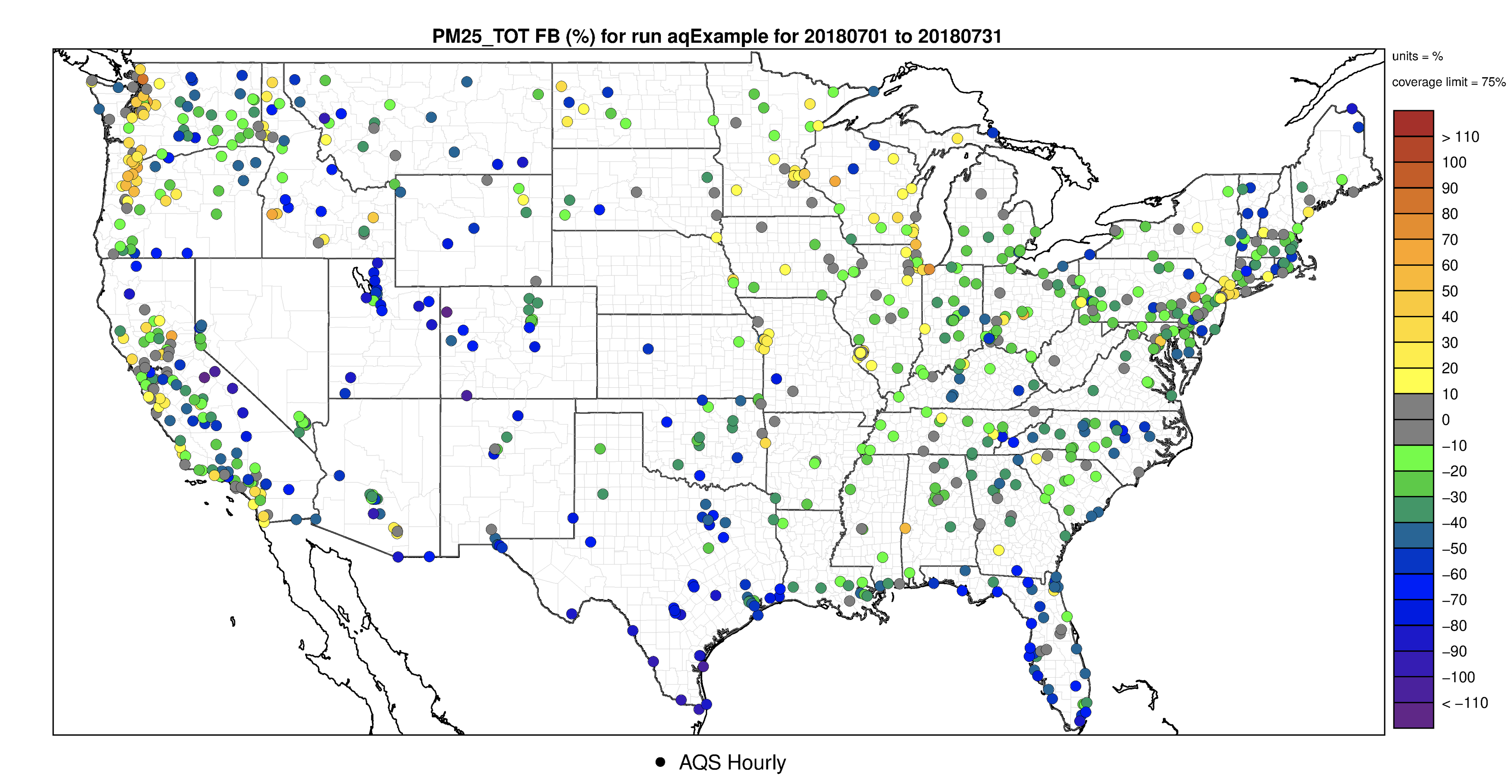
7.8.1. Create PM2.5 Spatial Plots

• Choose database
• select amet
• Choose project 1
  • select aqExample

• Under AQ Observation Networks
  • Select AQS - Hourly (e.g. NO,NO2,NOx,NOy,SO2,CO,PM2.5,O3,etc.)

• Under Species to Plot
  • Select PM25_TOT

• Under Date and Time Criteria
  • Select Start Date
  • Year: 2018
  • Month: 07
  • Day: 01
  • Select End Date
  • Year: 2018
  • Month: 07
  • Day: 31

• Under Choose Program to Run
  • Select Species Statistics and Spatial Plot(multi networks)

Select Run Program

Results of options selected in querygen_aq.php

PM2.5_TOT Normalized Mean Bias Plot

PM2.5_TOT Normalized Mean Error Plot

PM2.5_TOT Mean Bias Plot

PM2.5_TOT Mean Error Plot

PM2.5_TOT FBias Plot

PM2.5_TOT FError Plot

PM2.5_TOT RMSE Plot

PM2.5_TOT Correlation Plot

7.8.2. Interactive (Leaflet) Species Statistics and Spatial Plot

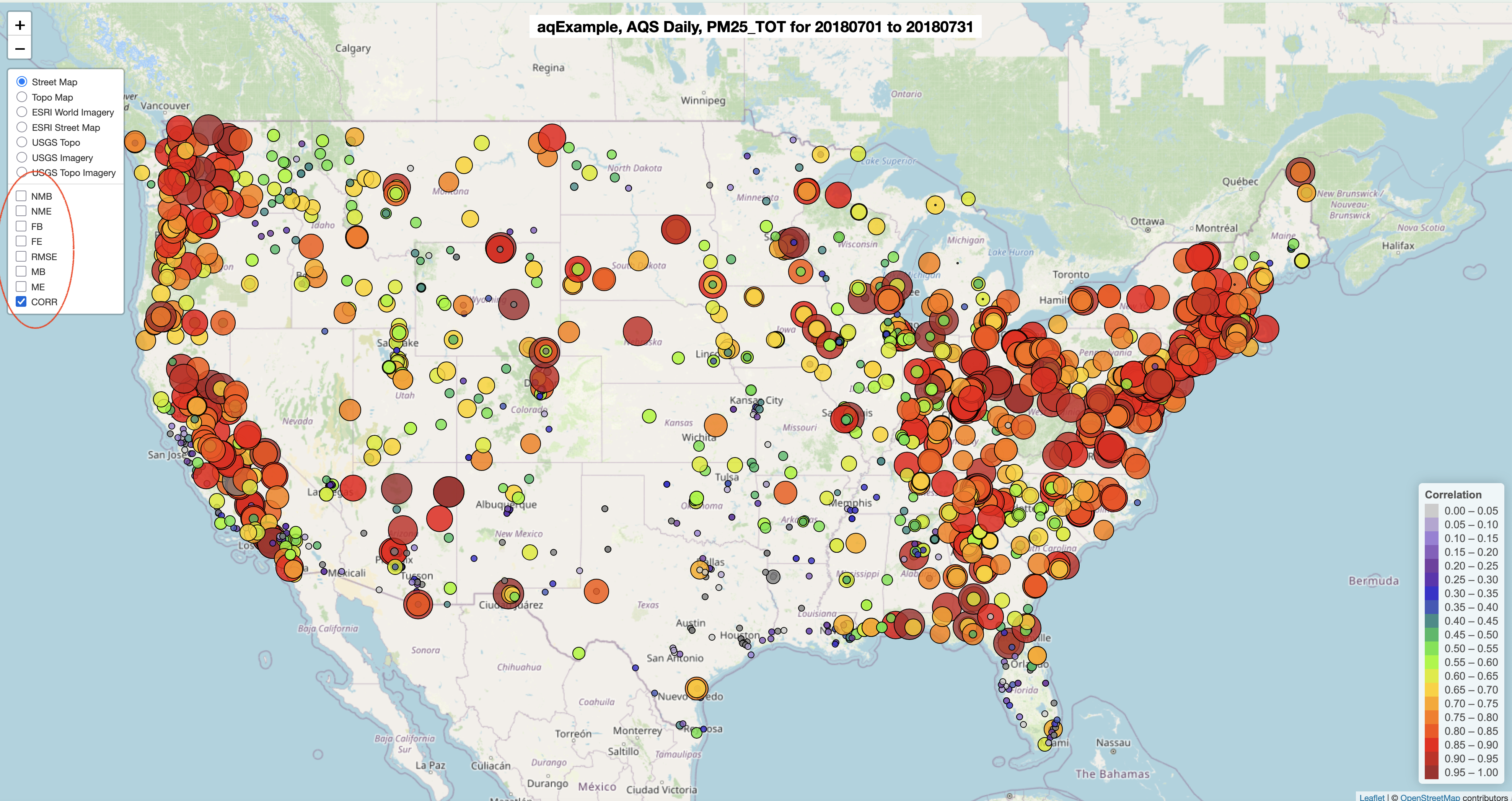
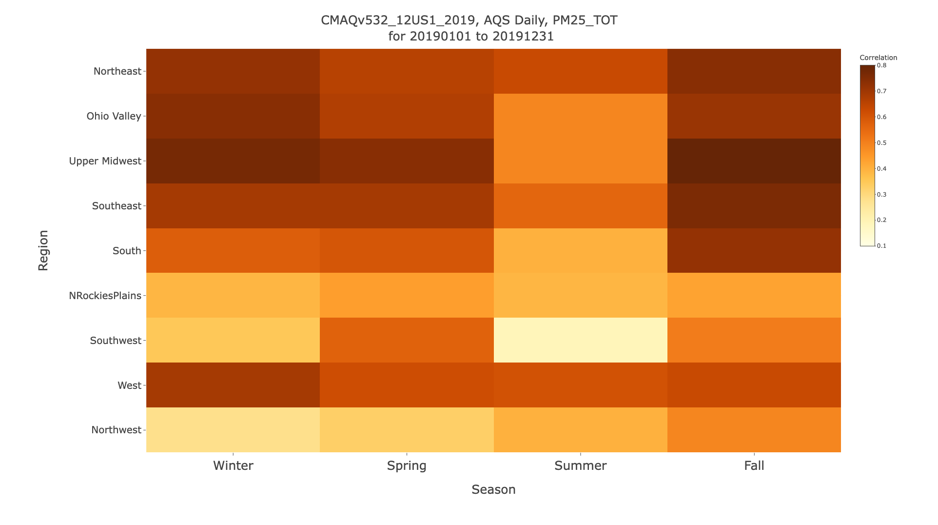
Run using the same project (aqExample), different observation network (AQS Daily) and same species (PM2.5_TOT) This creates a single plot with all metrics, use the legend to deselect every metric except the metric of interest (correlation (CORR) was chosen in this case).

PM2.5_TOT Correlation Plot using Leaflet Interactive Plot

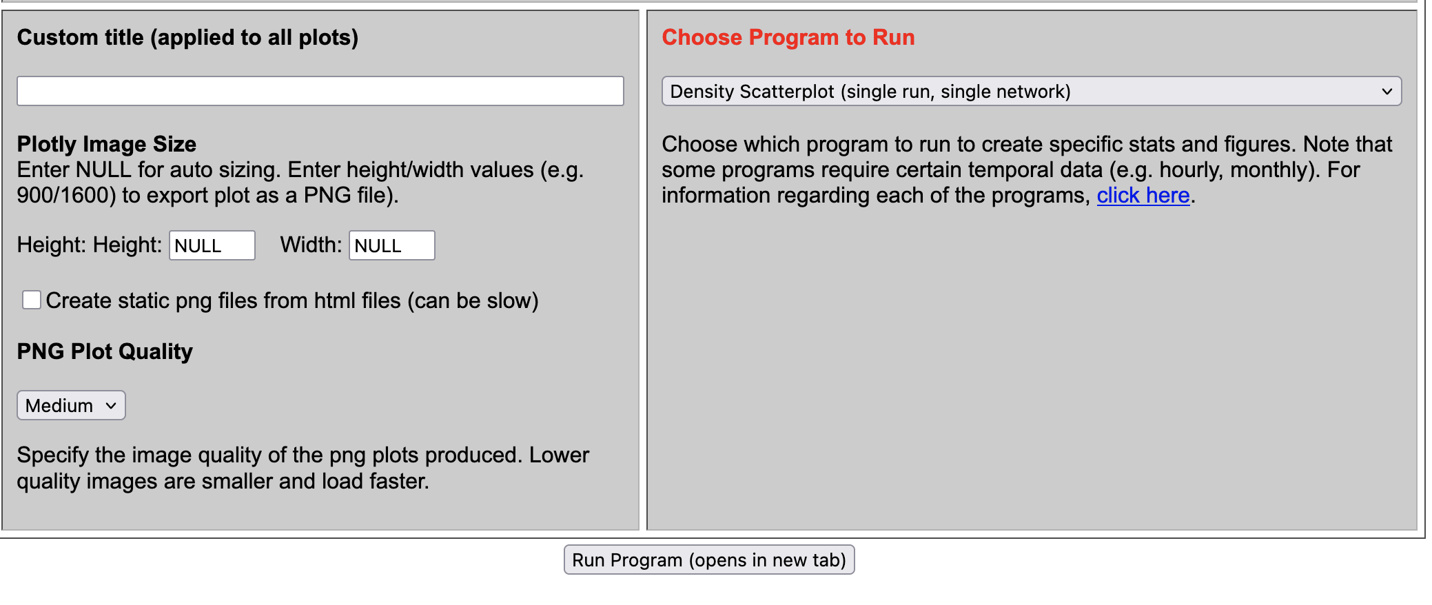
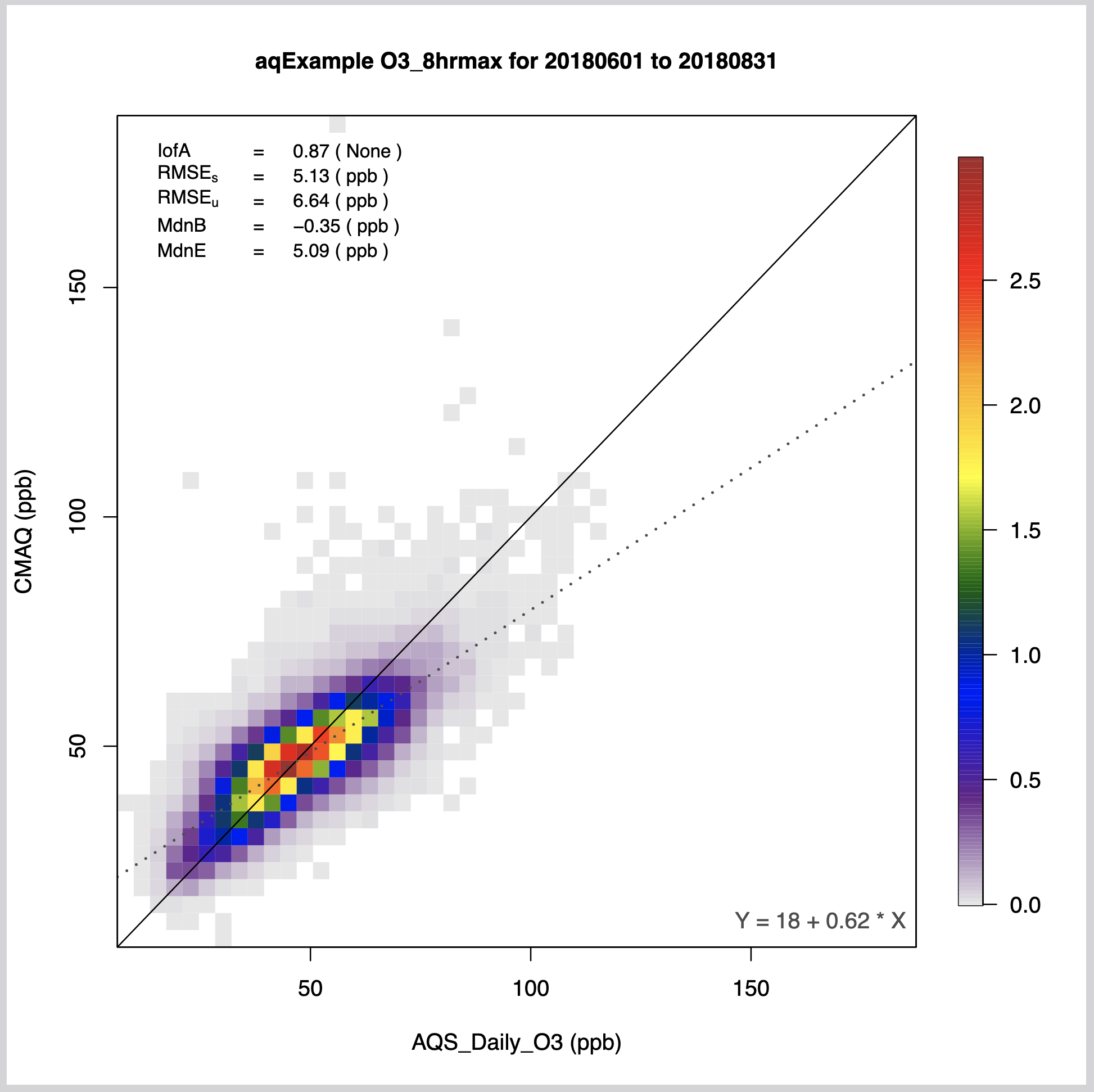
7.8.3. Create O3_8hrmax Density Scatterplot

• Under AQ Observation Networks
• Select AQS - Daily O3 (1-hr and 8-hr max) O3

• Under Species to Plot
• Select O3_8hrmax

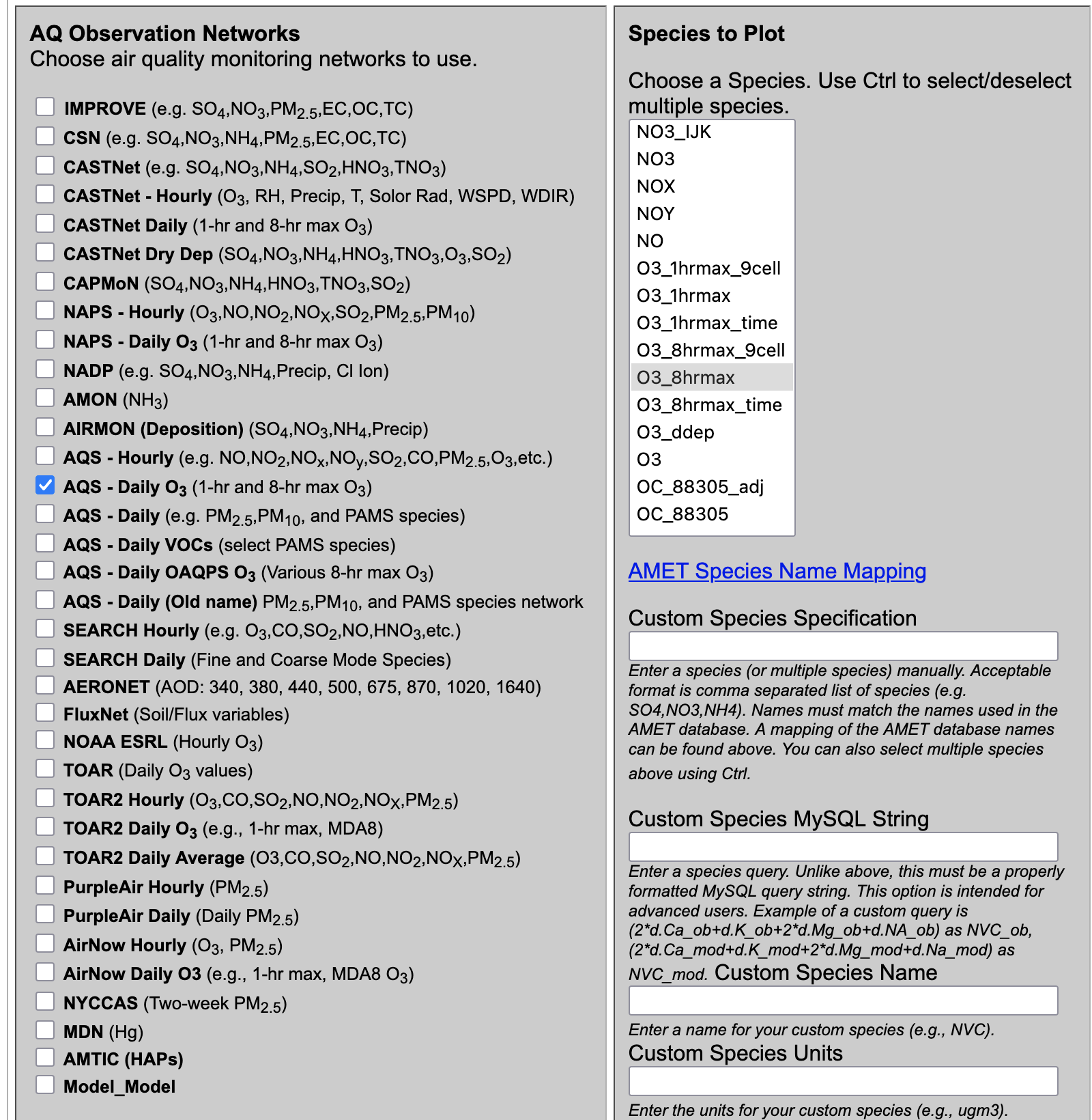
• Under Choose Program to Run
  • Select Density Scatterplot (single run, single network)

Results of options selected in querygen_aq.php form

Scatterplot of O3_8hrmax

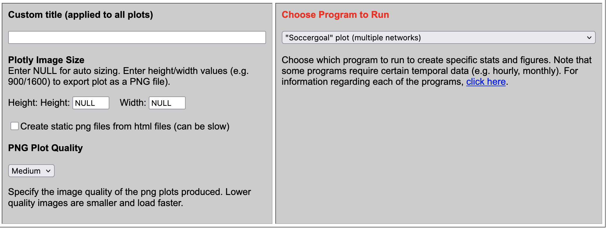
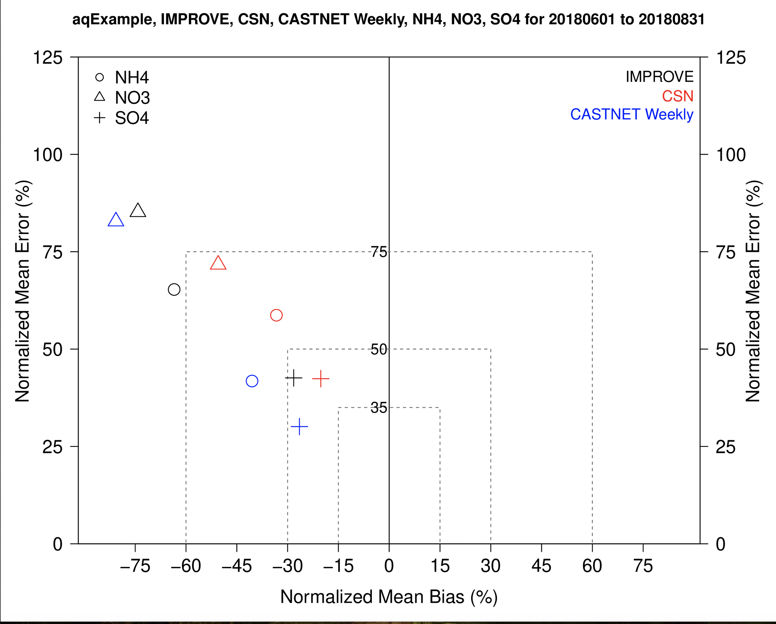
7.8.4. Create Soccerplot using Multiple Obs Networks, Multiple Species

• Under AQ Observation Networks
  • Select IMPROVE
  • Select CSN
  • Select CASTNet

• Under Species to Plot
  • Select SO4
  • Select NO3
  • Select NH4

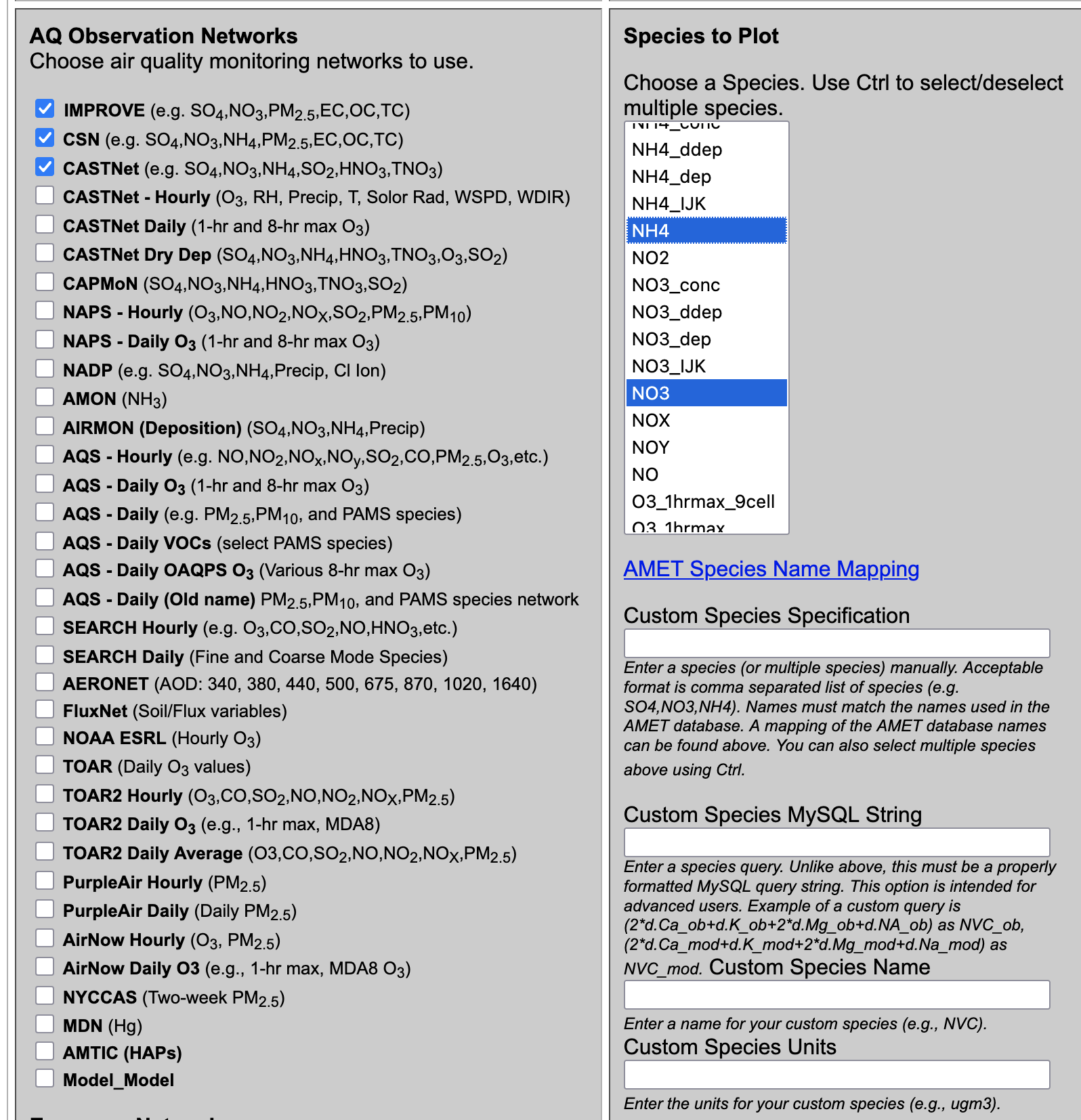
• Under Choose Program to Run
  • Select Soccergoal Plot (multiple networks)

Results of querygen_aq.php (links)

Soccerplot Generated

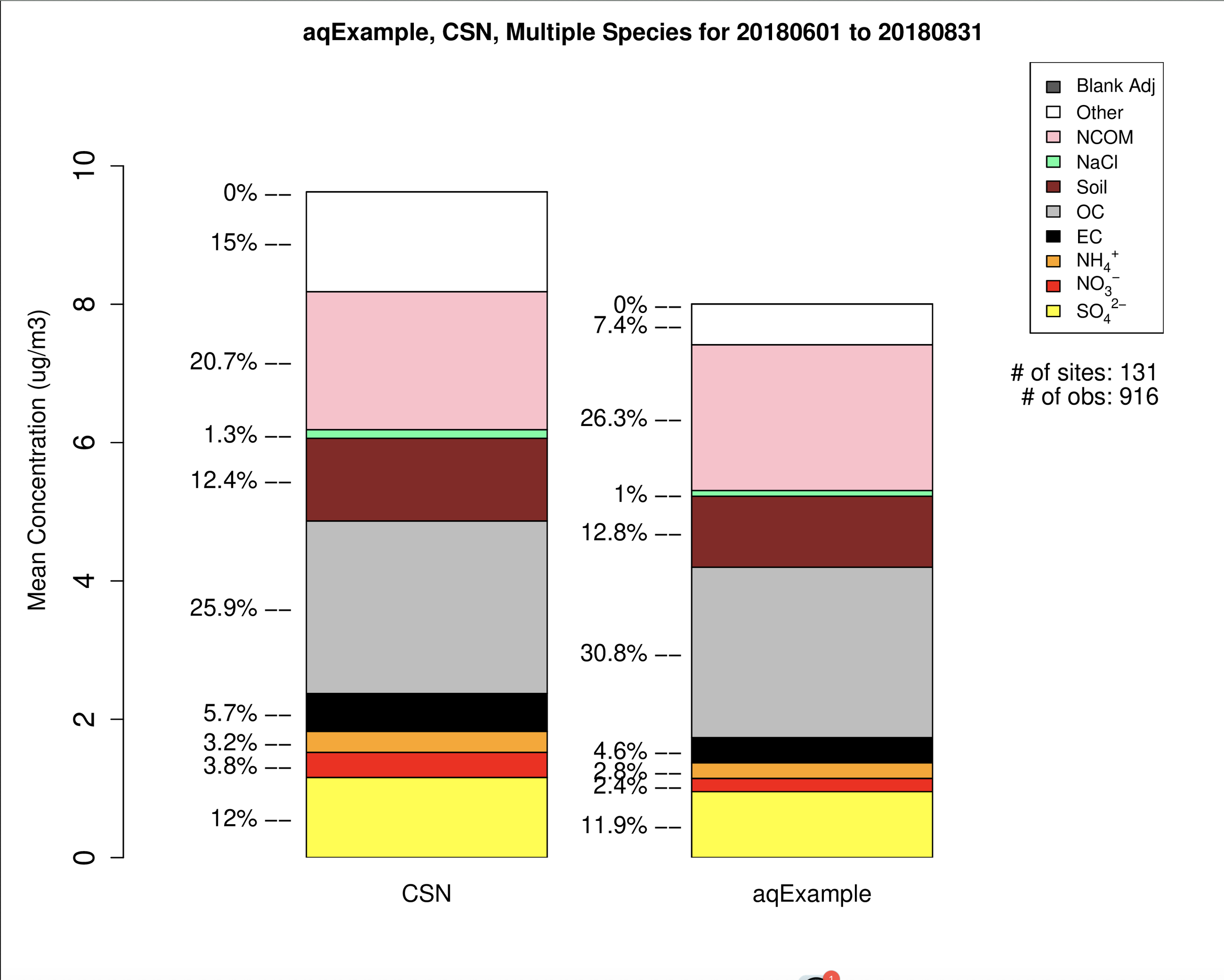
7.8.5. Create Stacked Bar Plot using CSN Network for PM2.5

• Under Observation Network
  • Select CSN

• Under Species to Plot
  • Select PM25_TOT

• Under Choose Program to Run
  • Select PM2.5 Stacked Bar Plot AE6 (CSN or IMPROVE, multirun)

Results of querygen_aq.php (links)

Stacked Bar Plot of PM2.5 using CSN Network

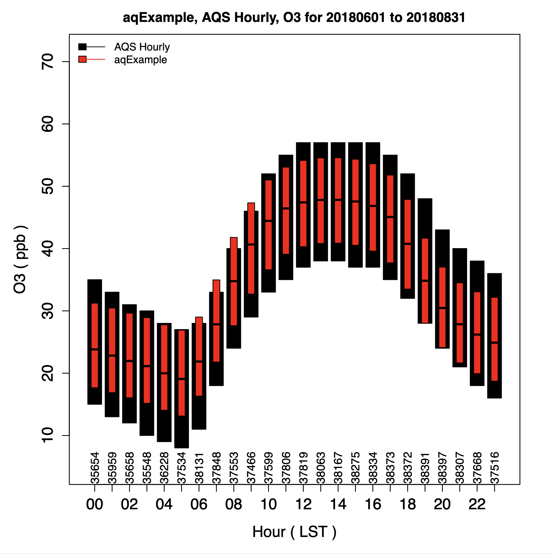
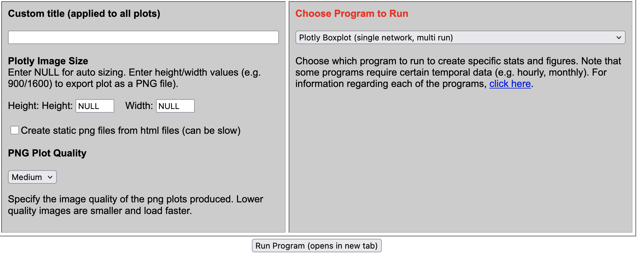
7.8.6. Create Hourly Boxplot using AQS Hourly and O3 Species

• Under Observation Network
  • Select AQS Hourly

• Under Species to Plot
  • Select O3

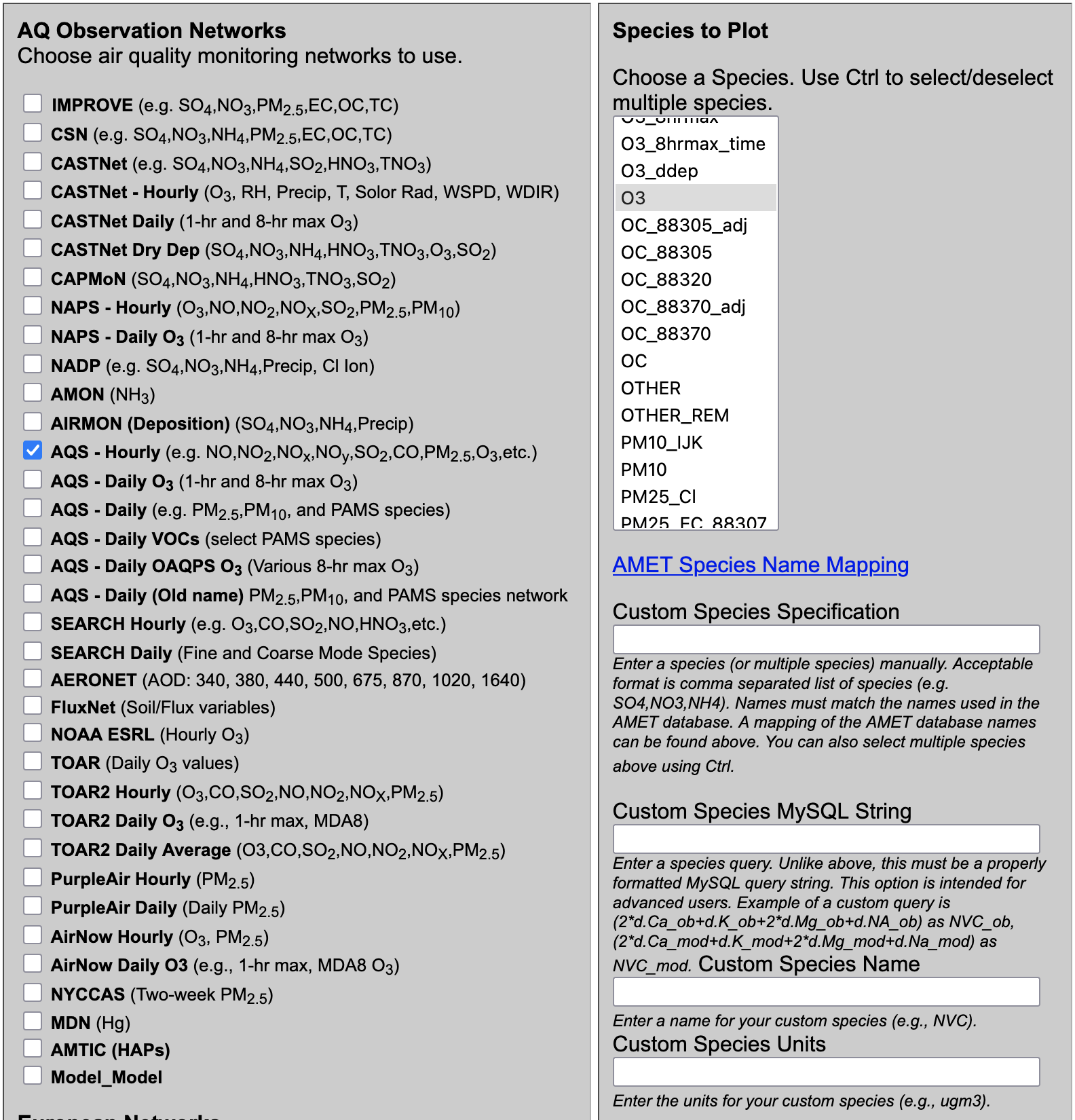
• Under Choose Program to Run
  • Select Hourly Boxplot (single network, multiple runs)

Hourly Boxplot of O3

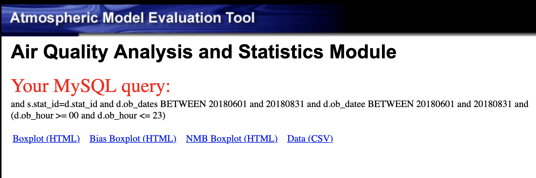
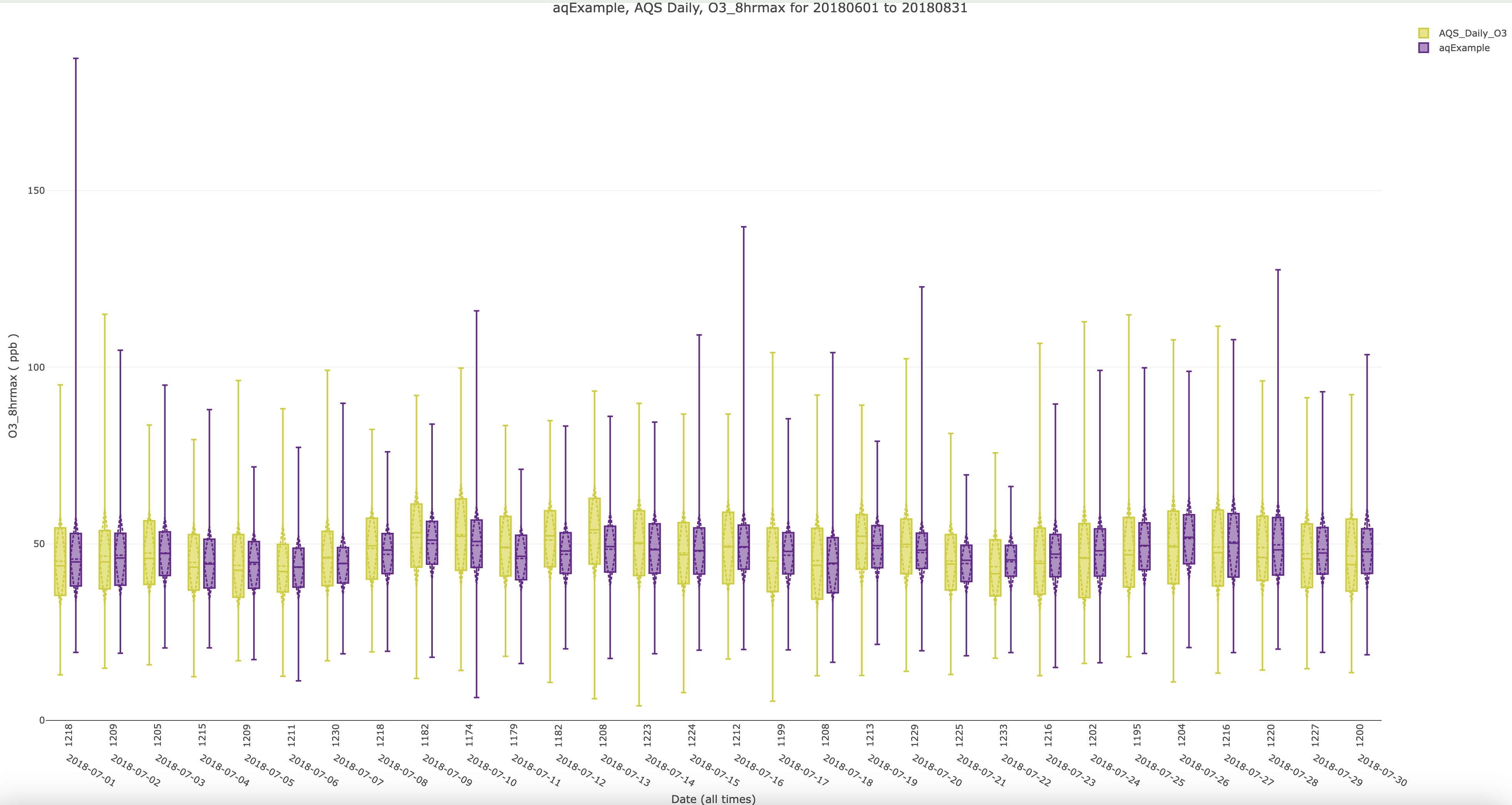
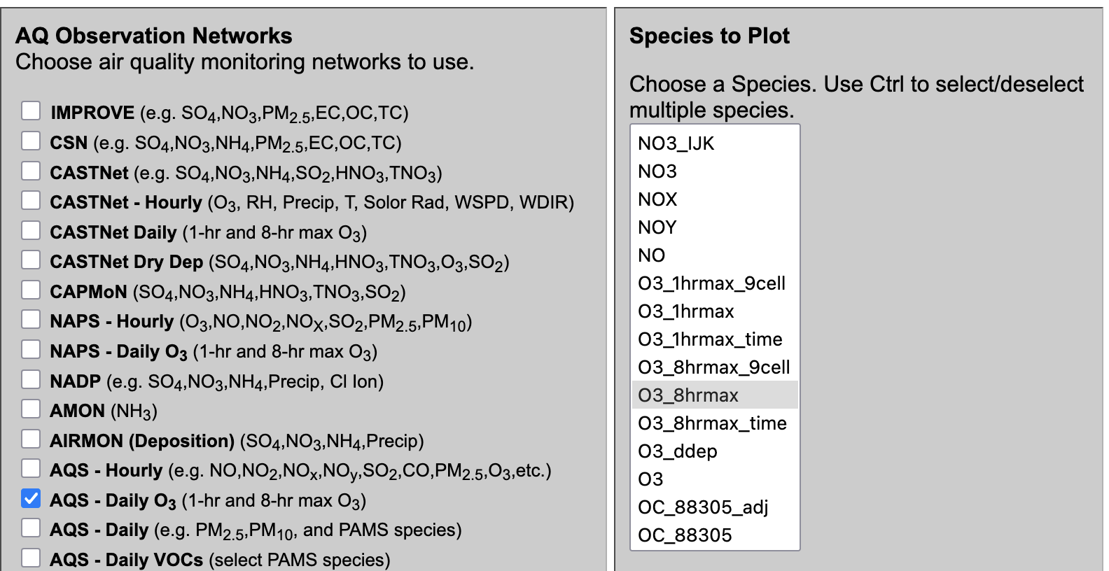
7.8.7. Create Daily Boxplot using AQS Daily and O3_8hrmax Species

• Under Observation Network
  • AQS - Daily O3 (1-hr and 8-hr max O3)

• Under Species to Plot
  • Select O3_8hrmax

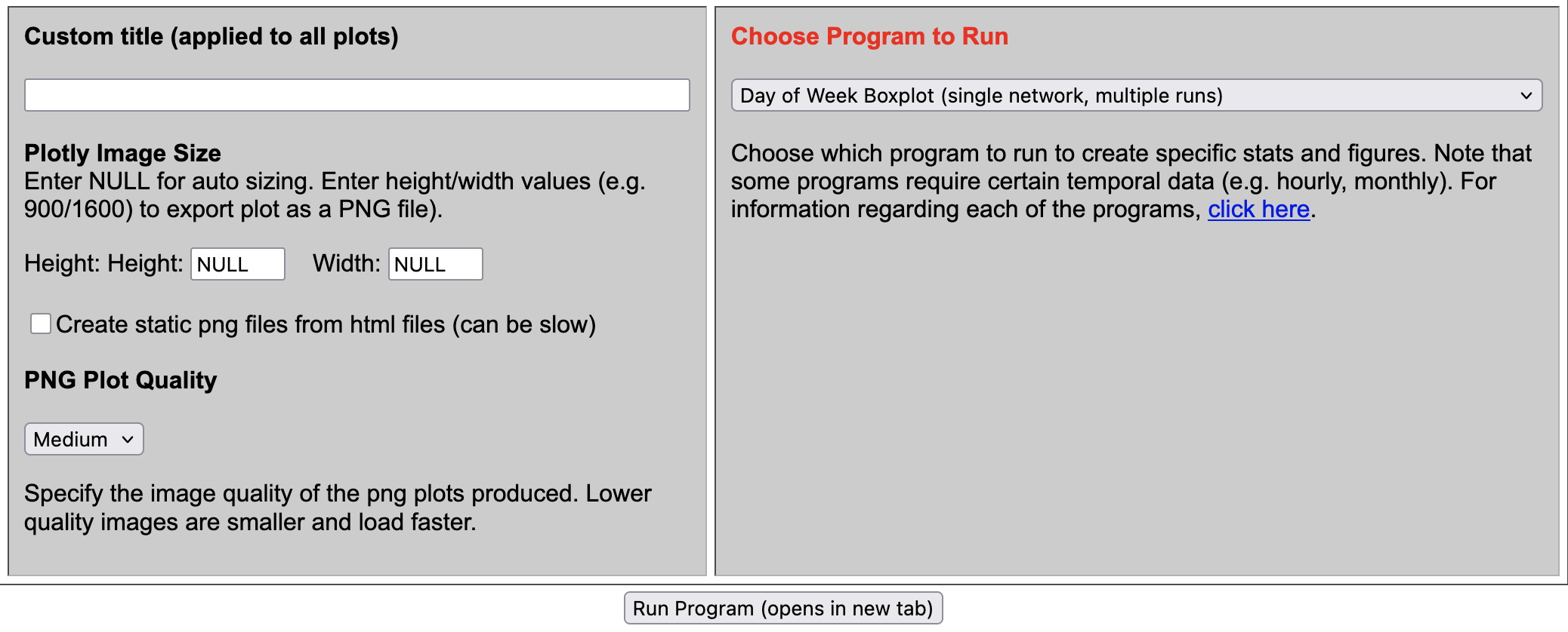
• Under Choose Program to Run
  • Select Plotly Boxplot (single network, multiple runs)

Query result

Daily Boxplot of O3_8hrmax

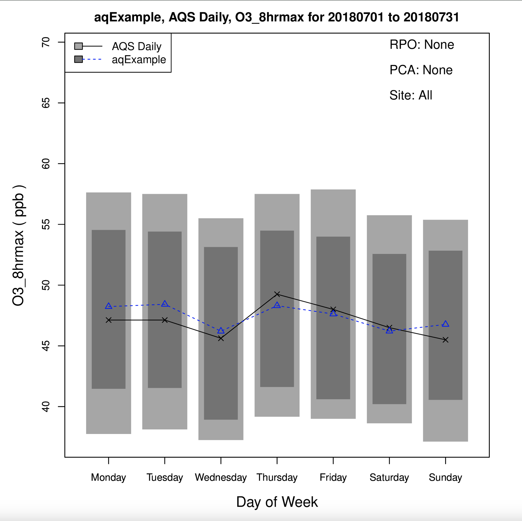
7.8.8. Create Day of Week (DoW) Boxplot using AQS Daily and O3_8hrmax Species

• Under Observation Network
  • Select AQS Daily O3 (1-hr and 8-hr max O3)

• Under Species to Plot
  • Select O3_8hrmax

• Under Choose Program to Run
  • Select Day of Week Boxplot (single network, multiple runs)

Day of Week (DoW) Boxplot of O3

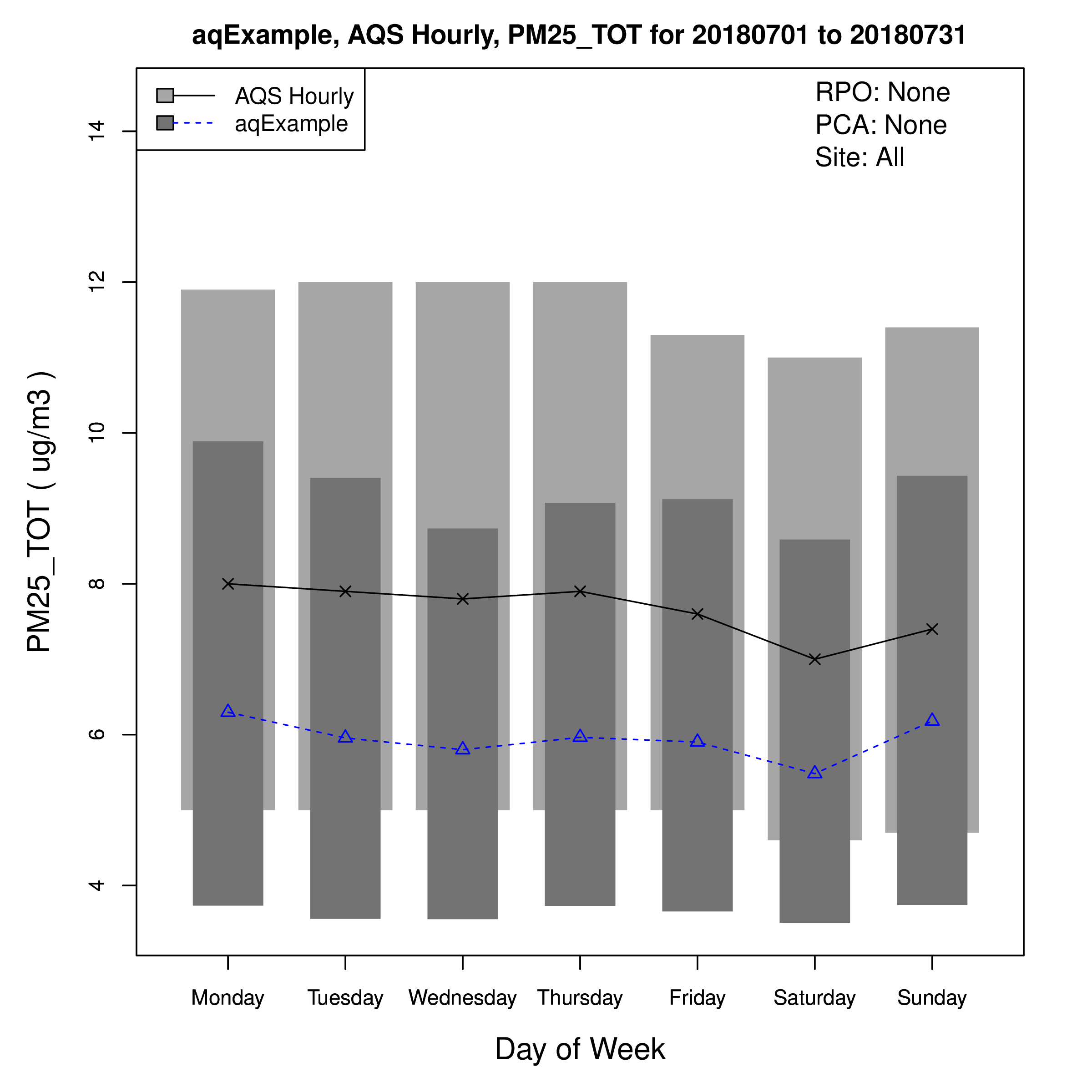
7.8.9. Create Day of Week (DoW) Boxplot using AQS Hourly and PM25_TOT

• Under Observation Network
  • Select AQS Hourly)

• Under Species to Plot
  • Select PM25_TOT

• Under Choose Program to Run
  • Select Day of Week Boxplot (single network, multiple runs)

Day of Week (DoW) Boxplot of PM25_TOT

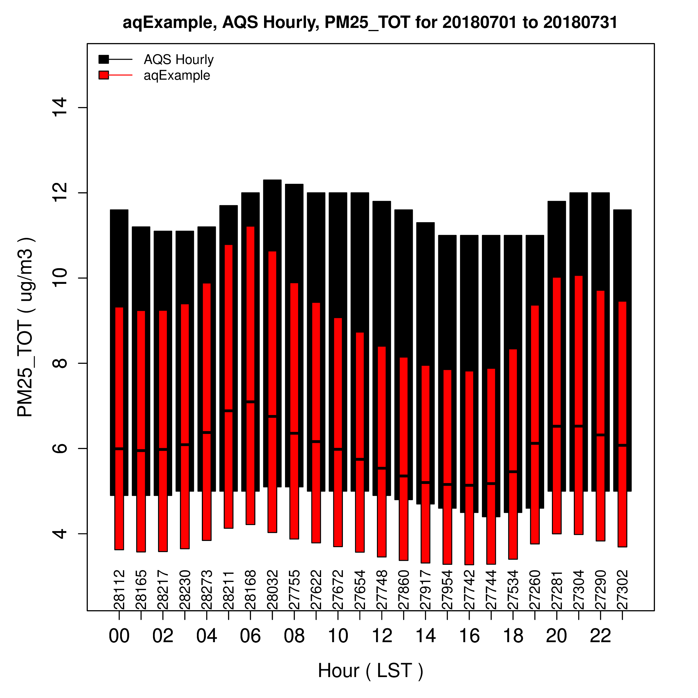
7.8.10. Create Hour of Day (Hourly) Boxplot using AQS Hourly and PM25_TOT

• Under Observation Network
  • Select AQS Hourly)

• Under Species to Plot
  • Select PM25_TOT

• Under Choose Program to Run
  • Select Hourly Boxplot (single network, multiple runs)

Hourly Boxplot of PM25_TOT

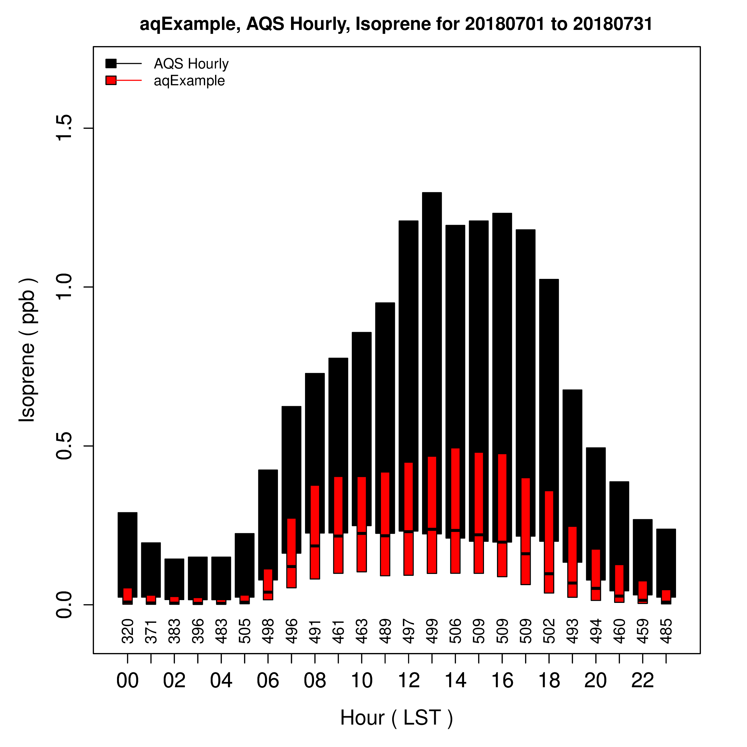
7.8.11. Create Hour of Day (Hourly) Boxplot using AQS Hourly and Isoprene

• Under Observation Network
  • Select AQS Hourly)

• Under Species to Plot
  • Select Isoprene

• Under Choose Program to Run
  • Select Hourly Boxplot (single network, multiple runs)

Hourly Boxplot of Isoprene

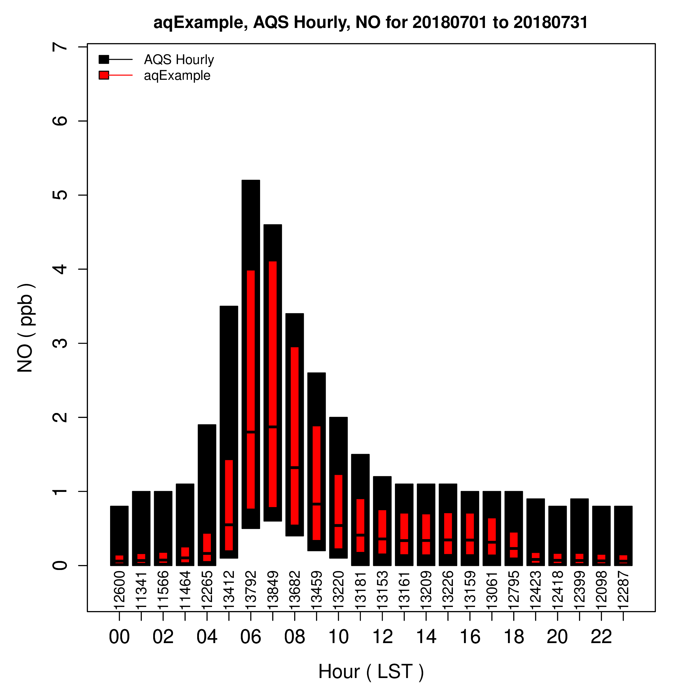
7.8.12. Create Hour of Day (Hourly) Boxplot using AQS Hourly and NO

• Under Observation Network
  • Select AQS Hourly)

• Under Species to Plot
  • Select NO

• Under Choose Program to Run
  • Select Hourly Boxplot (single network, multiple runs)

Hourly Boxplot of NO

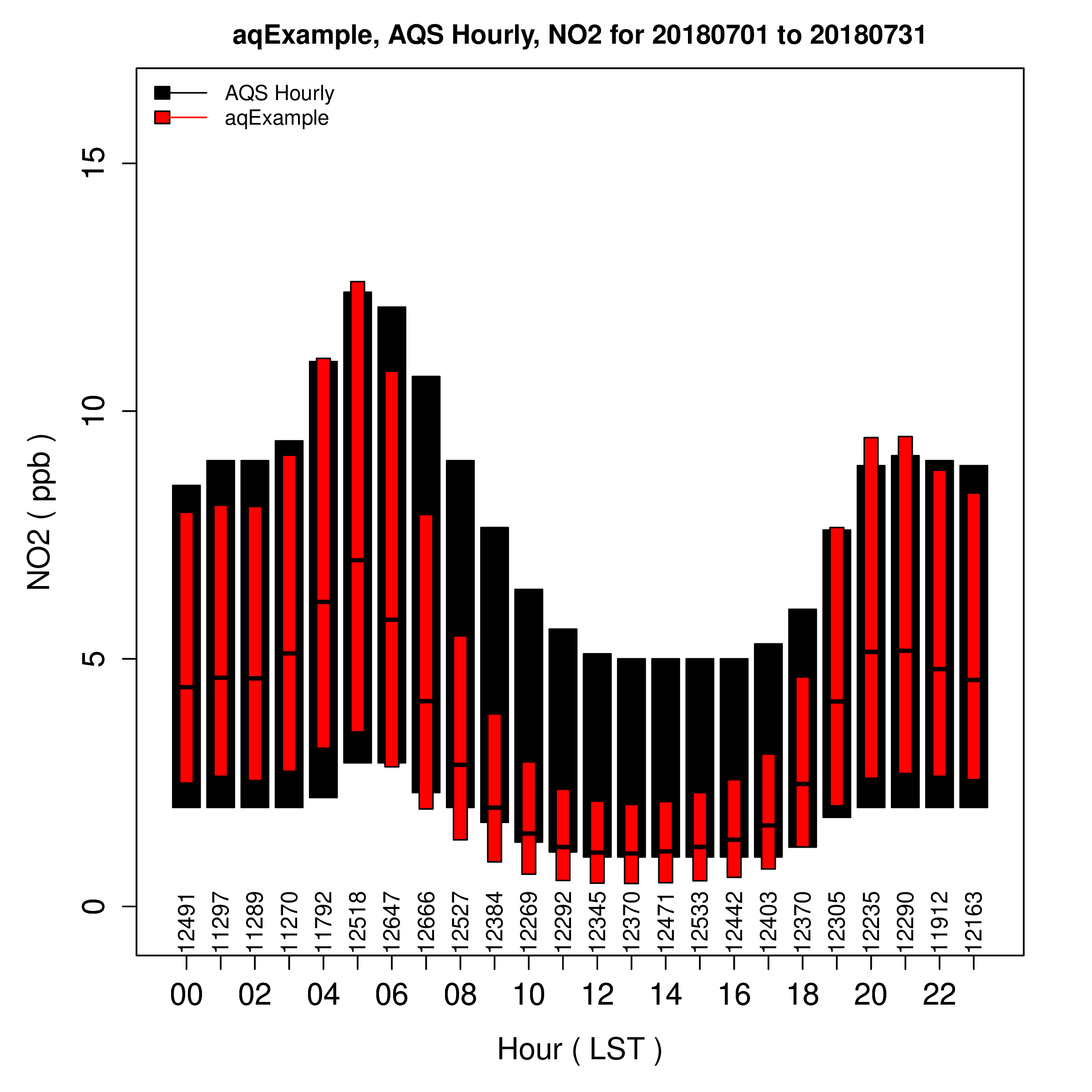
7.8.13. Create Hour of Day (Hourly) Boxplot using AQS Hourly and NO2

• Under Observation Network
  • Select AQS Hourly)

• Under Species to Plot
  • Select NO2

• Under Choose Program to Run
  • Select Hourly Boxplot (single network, multiple runs)

Hourly Boxplot of NO2

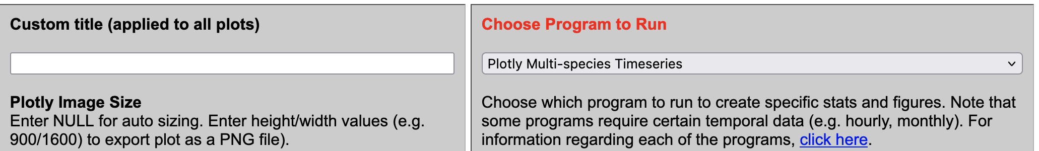
7.8.14. Create Interactive Hourly Timeseries using Plotly

• Under Observation Network
  • Select AQS Hourly

• Under Species to Plot
  • Select O3
  • Select NOX

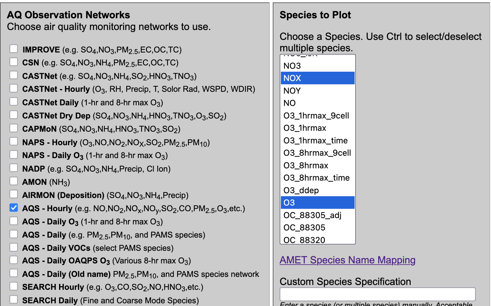
• Under Choose Program to Run
  • Choose Plotly Multi-species Timeseries

• Plotly Timeseries of O3 and NOX
  

Note, this plot is interactive, and you can turn off items by clicking on an item in the legend, and also window to a specific time within the plot.

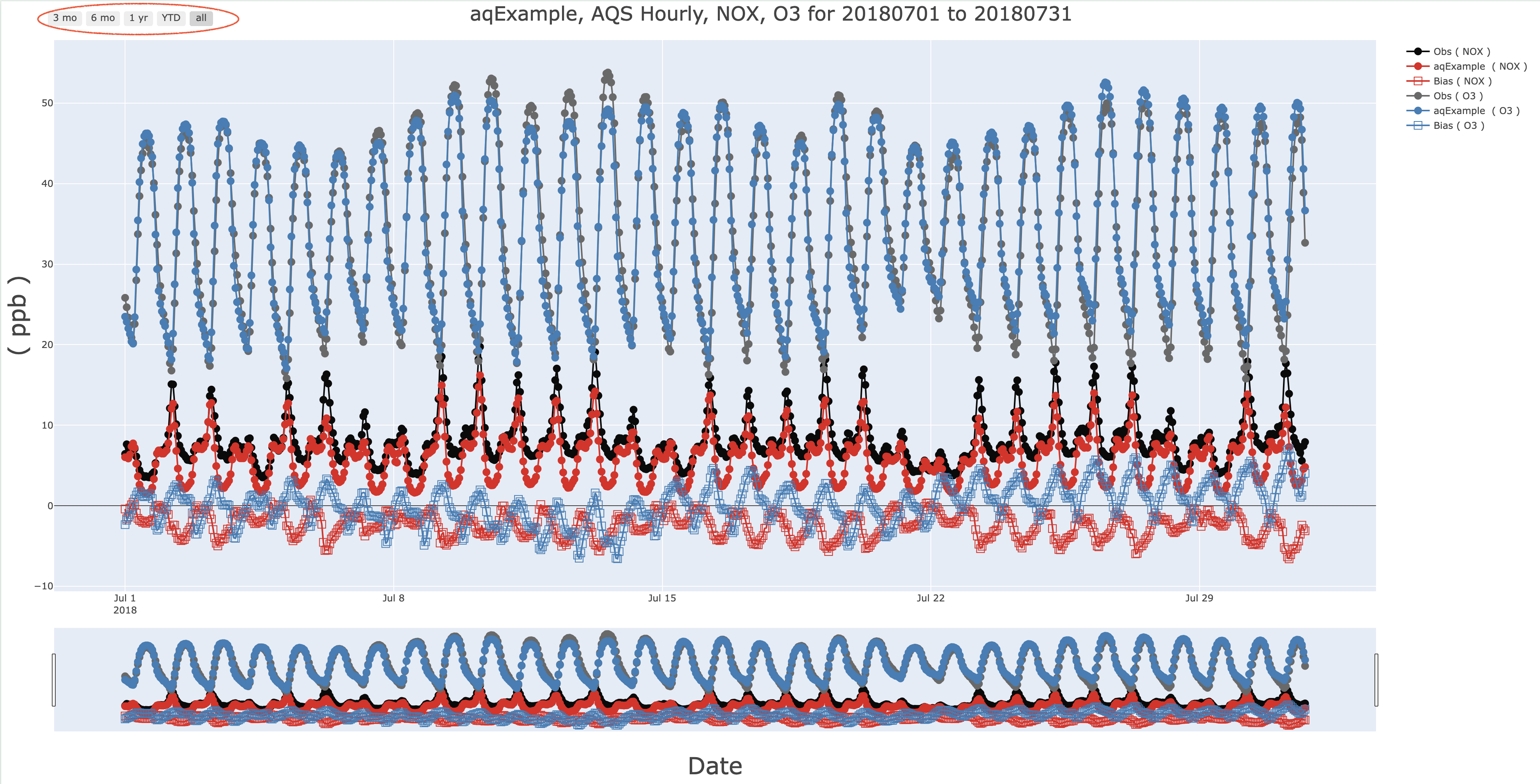
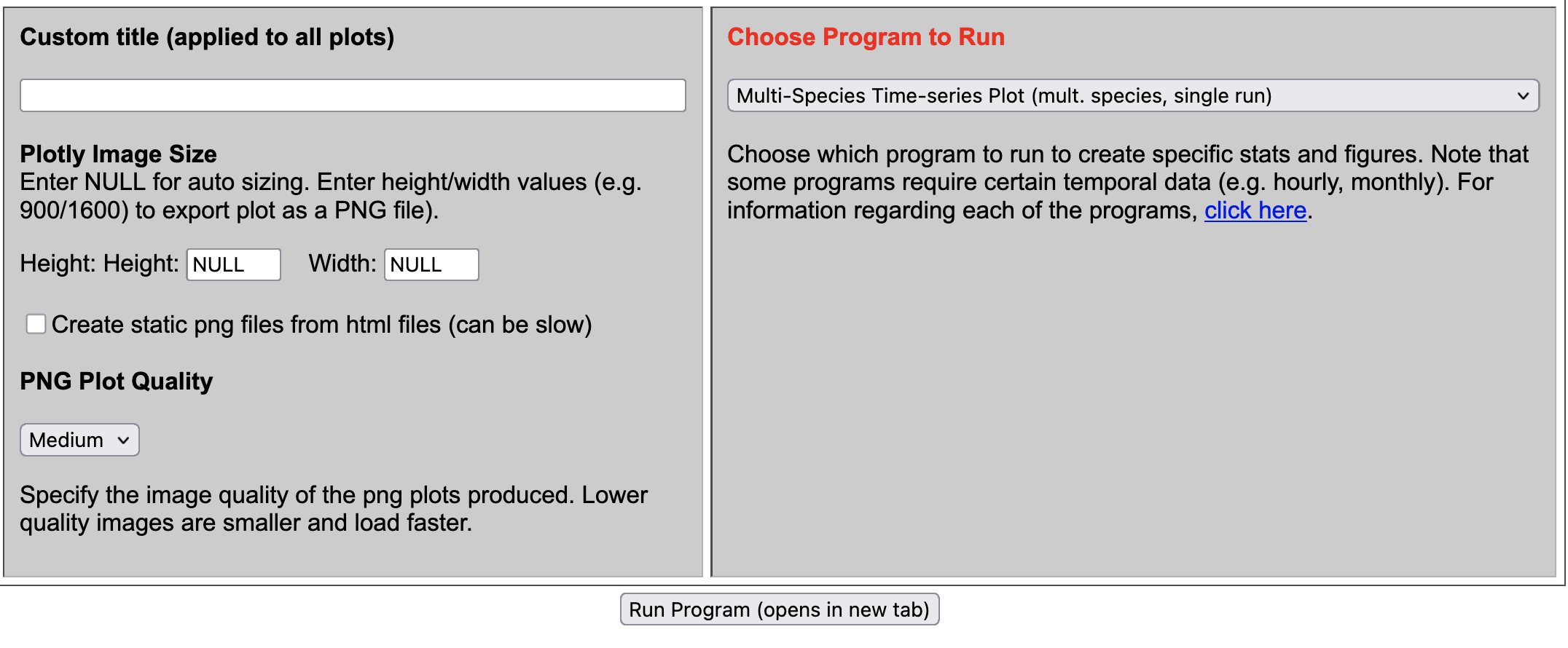
7.8.15. Create Multi-species Timeseries Plot

• Under Observation Network
  • Select AQS Hourly

• Under Species to Plot
  • Select O3
  • Select NOX

• Under Choose Program to Run
  • Choose Plotly Multi-species Timeseries

• Multispecies Timeseries of O3 and NOX and Bias Timeseries
  

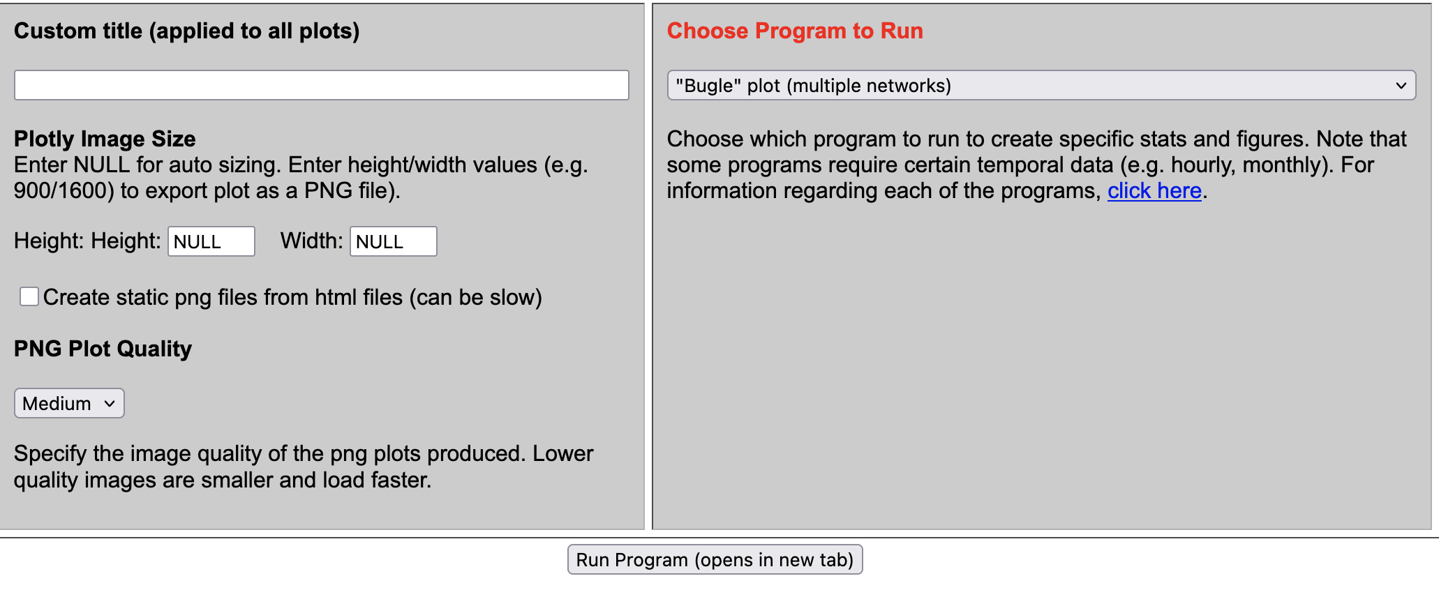
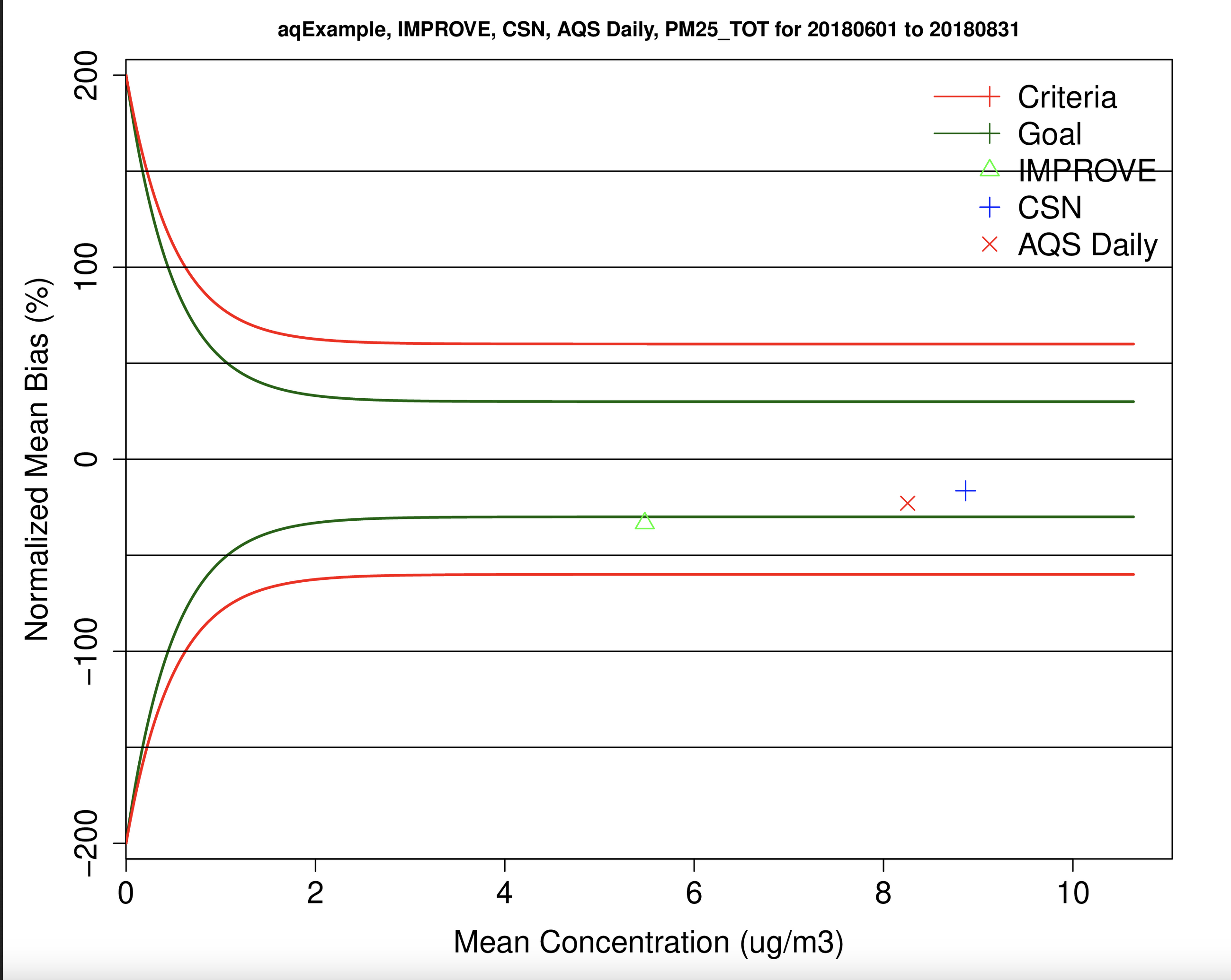
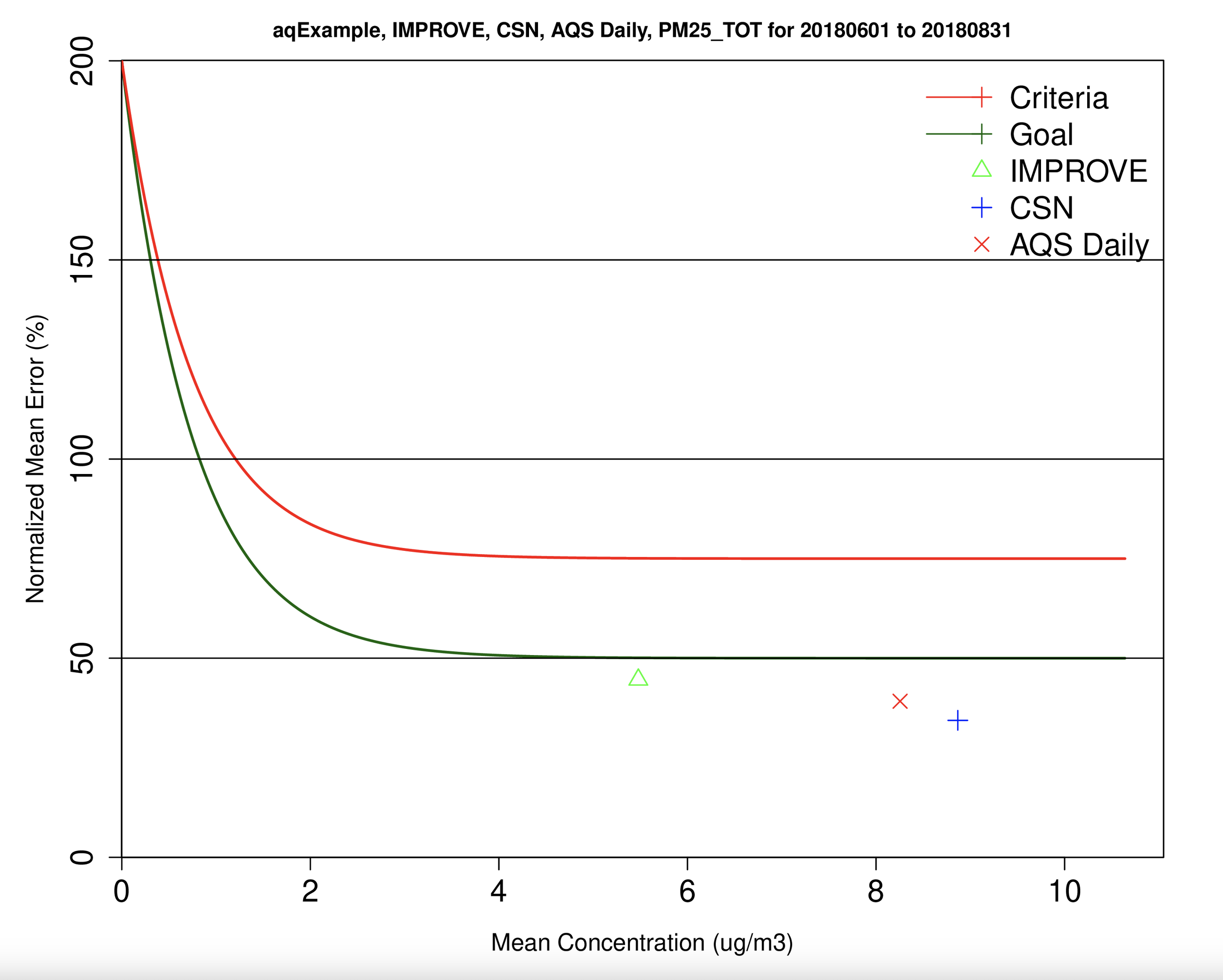
7.8.16. Create Bugle Plot of PM2.5_TOT for AQS Daily, CSN, and IMPROVE

• Under Observation Network
  • Select AQS Daily
  • Select CSN
  • Select IMPROVE

• Under Species to Plot
  • `Select PM25_TOT`

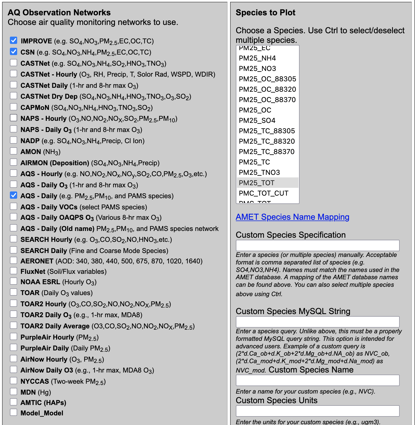
• Under Choose Program to Run
  • Choose Bugle Plot(Multiple Networks) under Misc Scripts

Bugle Plot of Normalized Mean Bias (NMB) PM25_TOT for Networks AQS Hourly and AQS Daily

Bugle Plot of Normalized Mean Error (NME) PM25_TOT for Networks AQS Hourly and AQS Daily

7.9. Load your own AQ model data to MariaDB

7.9.1. Prepare to load your own data

Load modules

Change to the c-shell

csh

Check modules available

module avail

Load Modules

module load ioapi-3.2/gcc-13.3  netcdf/gcc-13.3  openmpi/gcc  

Review directory set-up for files on /home/ubuntu

ls -lrt

total 48
drwxrwxr-x  3 ubuntu ubuntu 4096 Sep 23 16:43 Modules
drwxr-xr-x  3 ubuntu ubuntu 4096 Sep 23 18:15 aws
drwxrwxr-x 10 ubuntu ubuntu 4096 Sep 24 17:35 CMAQ55plus_REPO
drwxrwxr-x  8 ubuntu ubuntu 4096 Sep 24 17:52 CMAQv5.5+
drwx------  4 ubuntu ubuntu 4096 Sep 25 14:39 snap
drwxrwxr-x  3 ubuntu ubuntu 4096 Sep 25 17:17 MariaDB
drwxrwxrwx 15 ubuntu ubuntu 4096 Sep 25 19:30 AMET_v16
drwxrwxr-x  3 ubuntu ubuntu 4096 Sep 25 20:44 LIBRARIES
-rw-rw-r--  1 ubuntu ubuntu  467 Sep 29 17:25 ports.conf
-rw-rw-r--  1 ubuntu ubuntu 4962 Nov  3 15:22 branch_differences
-rw-rw-r--  1 ubuntu ubuntu  445 Nov  3 16:29 readme

Review directory set-up for files on /shared/AMET_v16

/shared/AMET_v16% ls -rlt */*
model_data/MET:
total 24
drwxrwxr-x 2 ubuntu ubuntu  4096 Sep 23 22:58 metExample_wrf
drwxrwxr-x 2 ubuntu ubuntu  4096 Sep 23 23:58 metExample_mpas
drwxrwxr-x 3 ubuntu ubuntu 12288 Sep 25 12:54 metExample_mcip

model_data/AQ:
total 4
drwxrwxr-x 2 ubuntu ubuntu   40 Nov  3 17:25 aqExample

Review size of data on /shared/AMET_v16 (note this is a 1 TB volume)

du -sh
768G

Review size of data on /home/ubuntu

du -sh
46G	.

Review size of the file systems available

df -h
Filesystem       Size  Used Avail Use% Mounted on
/dev/root        290G   61G  230G  21% /
tmpfs            7.8G     0  7.8G   0% /dev/shm
tmpfs            3.1G  1.0M  3.1G   1% /run
tmpfs            5.0M     0  5.0M   0% /run/lock
efivarfs         128K  4.1K  119K   4% /sys/firmware/efi/efivars
/dev/nvme0n1p16  881M  151M  669M  19% /boot
/dev/nvme0n1p15  105M  6.2M   99M   6% /boot/efi
/dev/nvme1n1    1000G  787G  214G  79% /shared
tmpfs            1.6G   20K  1.6G   1% /run/user/1000

Note that AMET_Website is installed under /var/www/html

ls -rlt /var/www/html
total 724
-rw-rw-r-- 1 www-data www-data   4333 Sep 23 17:55 AMET_Species_Name_Mapping.txt
-rw-rw-r-- 1 www-data www-data    420 Sep 23 17:55 example_stat_file.txt
-rw-rw-r-- 1 www-data www-data   2283 Sep 23 17:55 disaq_4km_met_sites.txt
-rw-rw-r-- 1 www-data www-data    331 Sep 23 17:55 disaq_1km_met_sites.txt
-rw-rw-r-- 1 www-data www-data   2700 Sep 23 17:55 O3_NA_monitors_2018.txt
-rw-rw-r-- 1 www-data www-data   8434 Sep 23 17:55 O3_NAA_Sites_v2_short_names.txt
-rw-rw-r-- 1 www-data www-data   4257 Sep 23 17:55 O3_NAA_Sites_v2_no_names.txt
drwxrwxr-x 2 www-data www-data   4096 Sep 23 17:55 images
-rw-rw-r-- 1 www-data www-data   6475 Sep 23 17:55 run_info_met.template
-rw-r--r-- 1 www-data www-data  10671 Sep 25 18:41 index.html.back
-rw-rw-r-- 1 www-data www-data    286 Sep 25 19:47 index.html.sv
-rwxrwxr-x 1 www-data www-data 259423 Sep 29 18:30 querygen_met.php
-rw-rw-r-- 1 www-data www-data   3861 Oct 10 17:10 amet-lib.php
-rwxrwxr-x 1 www-data www-data   2061 Oct 10 17:24 amet-config.R
-rw-rw-r-- 1 www-data www-data   2084 Oct 10 17:27 amet-www-config.php
-rw-rw-r-- 1 www-data www-data  11397 Oct 10 17:30 run_info.template
-rwxrwxr-x 1 ubuntu   ubuntu   362697 Oct 10 19:58 querygen_aq.php
drwxrwxrwx 2 www-data www-data  16384 Nov  3 15:12 cache

7.9.2. Upload your data

Change to the directory on /shared volume

cd /shared/AMET_v16/model_data/AQ/ 
mkdir new_project

Use the s3 cp command to obtain your data

cd new_project
aws s3 --no-sign-request --region=us-east-1 cp --recursive s3://[your_project_bucket_name]

7.9.3. Load your project data into the database

Create a new project under the script_db directory

cd ~/AMET_v16/scripts_db/
cp -rp aqExample new_project
cd new_project
mv aqProject_pre_and_post.csh new_project_pre_and_post.csh

Modify the project name in the script

vi new_project_pre_and_post.csh

Change:
  set APPL      = aqExample         #> Application Name (e.g. Gridname)
to:
  set APPL      = new_project         #> Application Name (e.g. Gridname)

Edit the run description

Change:
 setenv RUN_DESCRIPTION "CMAQv5.5 AMET aqExample test case. July 2018."
to
 setenv RUN_DESCRIPTION "CMAQv5.5 AMET new project. Nov. 2025"

Edit the path to the combine output, if that is what you are uploading for your new_project.

Check if observation data is available.

cd ~/AMET_v16/obs
ls -lrt */*

Currently only the obsdata for 2018 has been copied from the s3 bucket to this location. Follow instructions on the readme file to copy additional years, and then extract them.

Once your model data and the observation data is available, run the net_project_pre_and_post.csh script.

7.10. Loading EPA’s EQUATES Database

This method was used to load the EQUATES Database to the EC2 instance.

Create the amad_EQUATES database using mysql

mysql CREATE DATABASE amad_EQUATES;

Imported the mysql dump provided by Wyat Appel using the following command.

sudo mysql -p amad_EQUATES < amad_EQUATES.dump & 

Verify the import by using the AMET Website to view all of the imported tables.

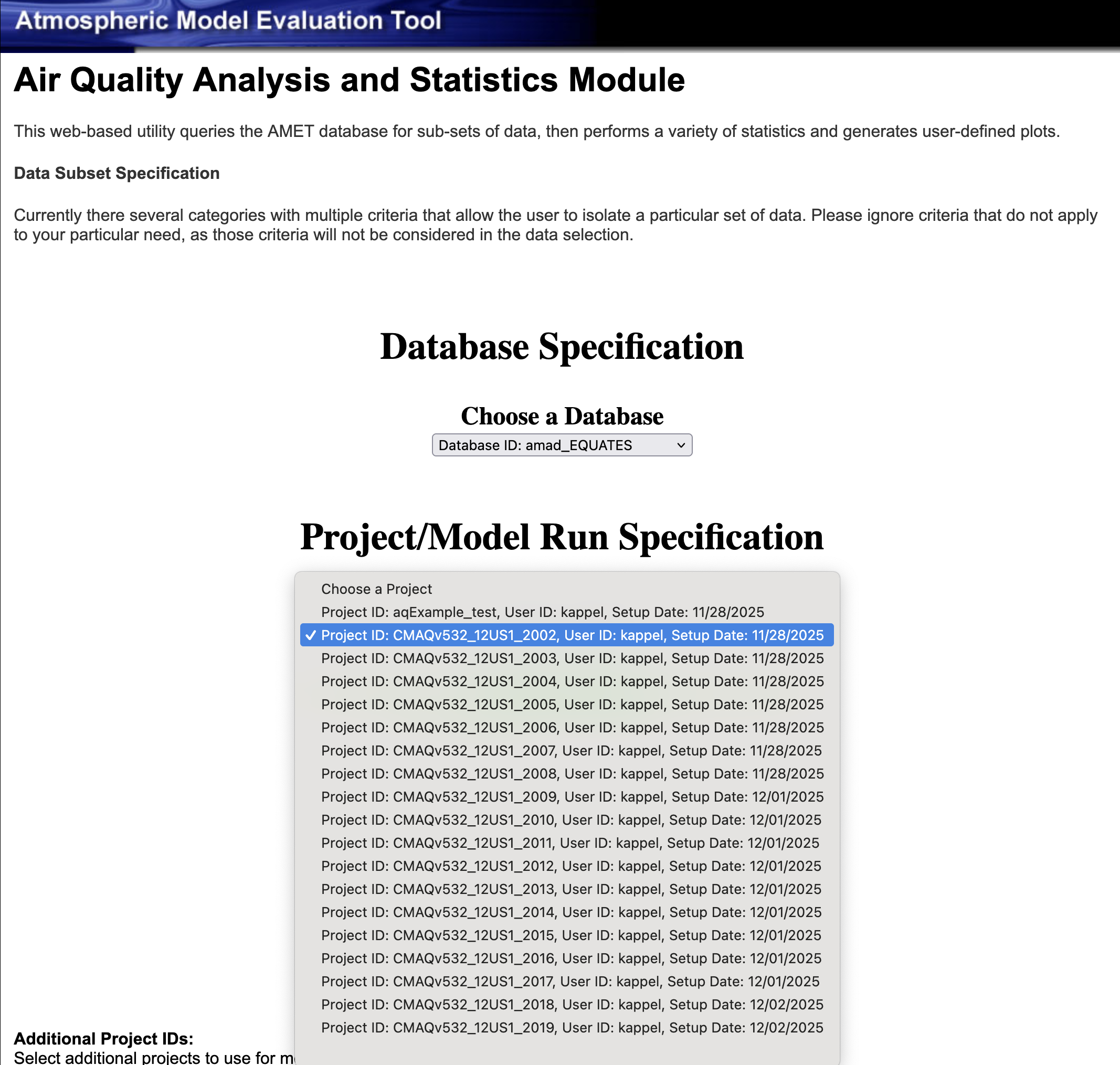
7.11. Example plots using the EQUATES 2002-2019 Projects in the amad_EQUATES database

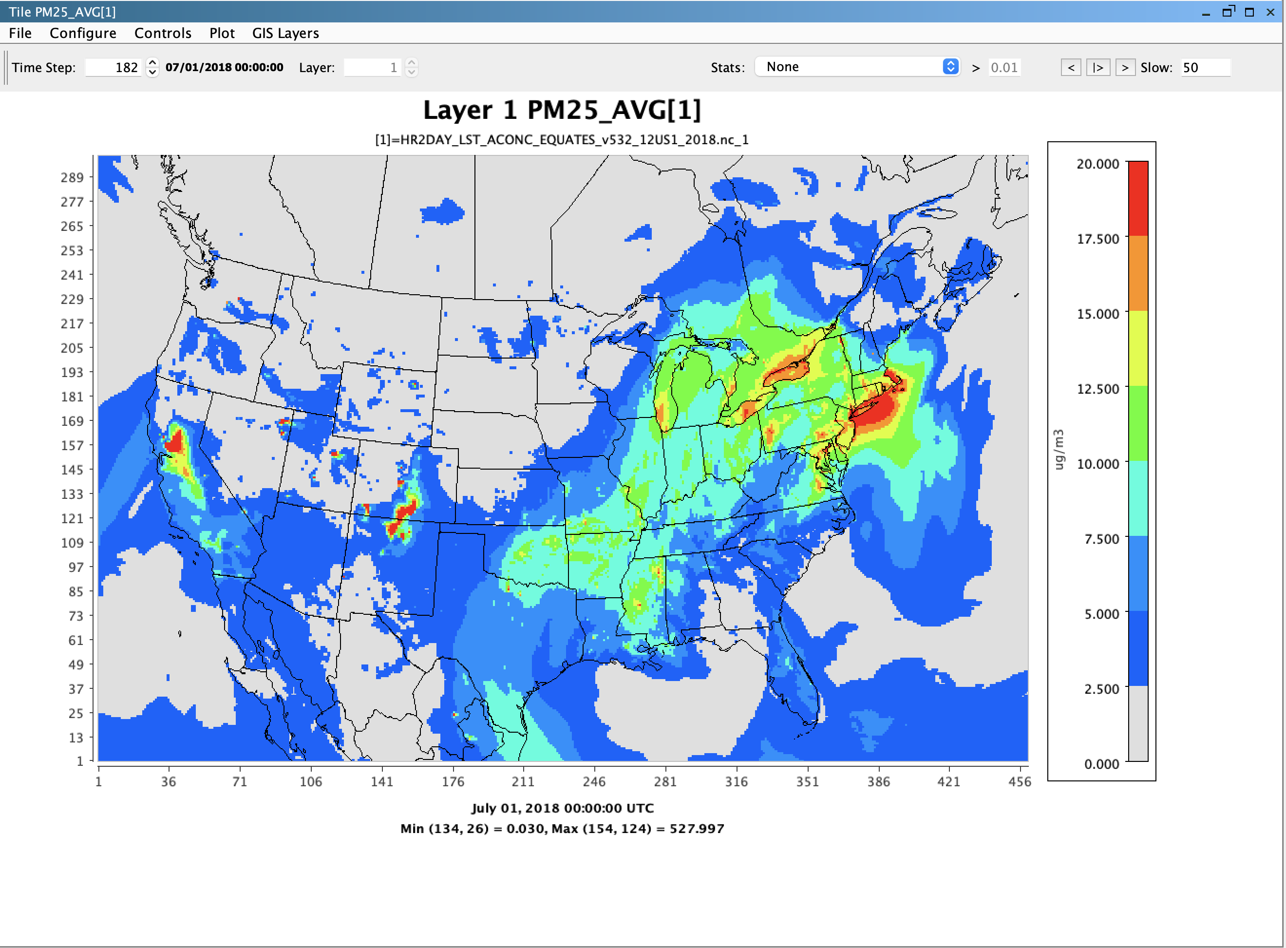
VERDI Plot of PM25_AVG (Daily Average) from HR2DAY_LST_ACONC_EQUATES_v532_12US1_2018.nc

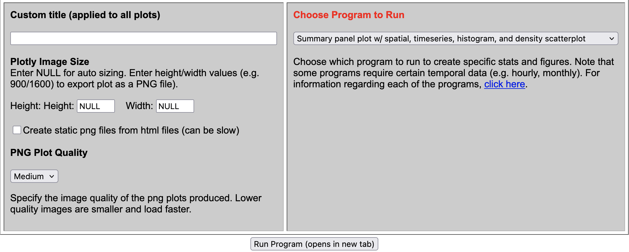
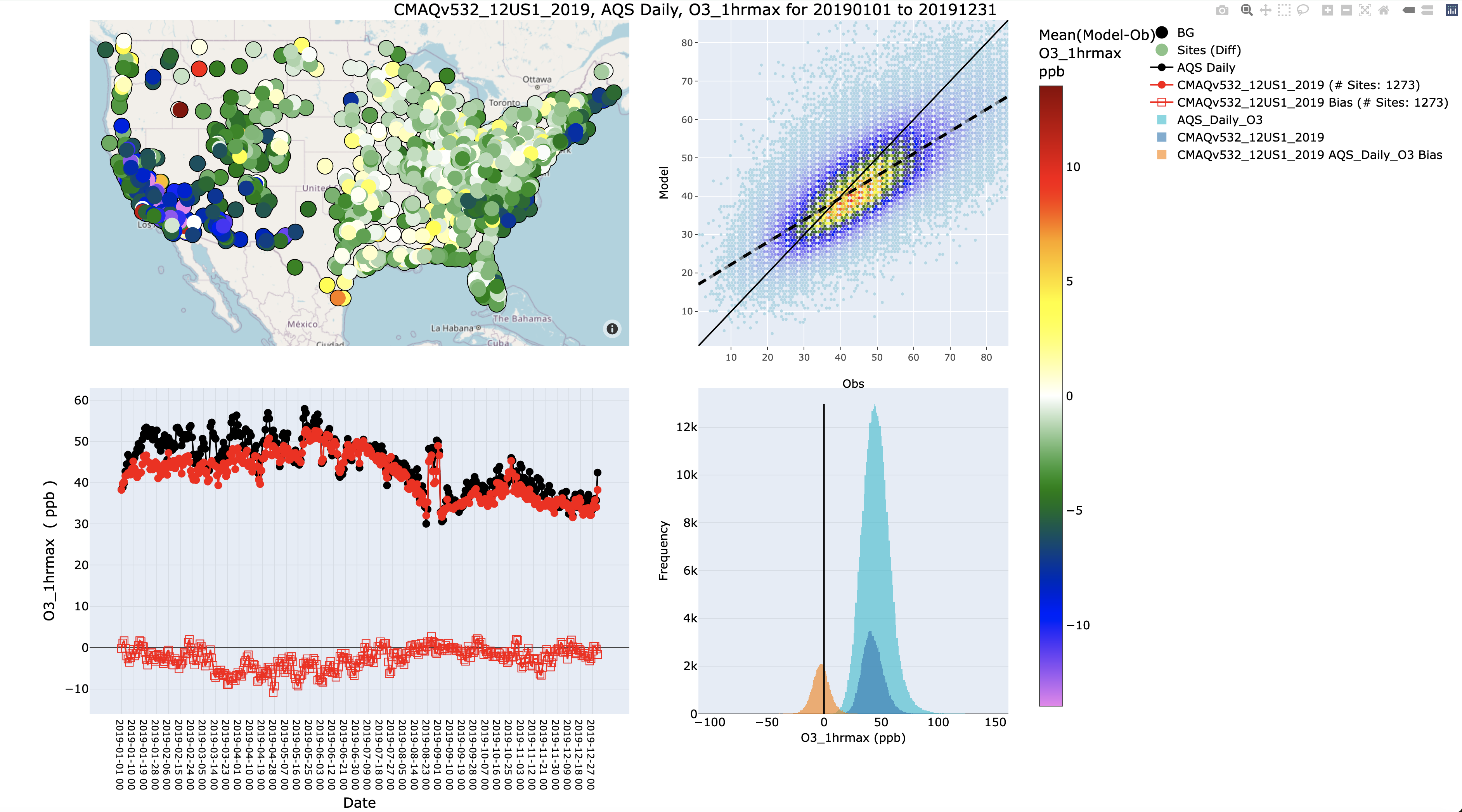
7.11.1. Create Summary Panel Plot w/ spatial, timeseries, histogram, and density scatterplot

• Select Database ID
  • Select amad_EQUATES

• Select Project ID
  • Select CMAQv532_12US1_2019

• Under Observation Network
  • Select AQS Daily O3

• Under Species to Plot
  • Select O3_1hrmax

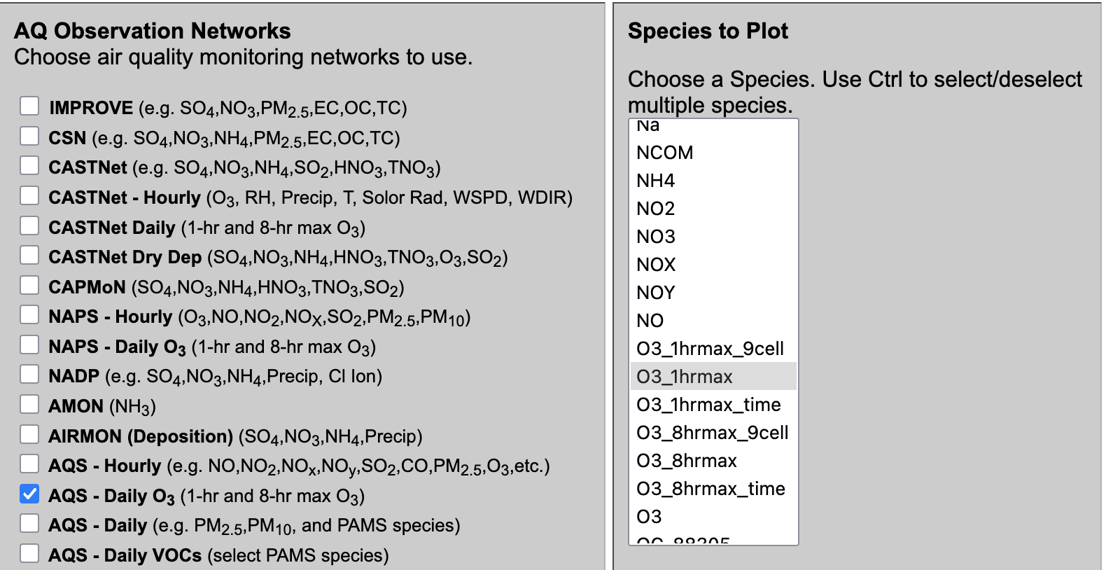
• Under Choose Program to Run
  • Summary panel plot w/spatial, timeseries, histogram, and density scatterplot

Summary Panel Plot w/ spatial, timeseries, histogram, and density scatterplot using Networks AQS Daily O3 and Ozone_1hrmax

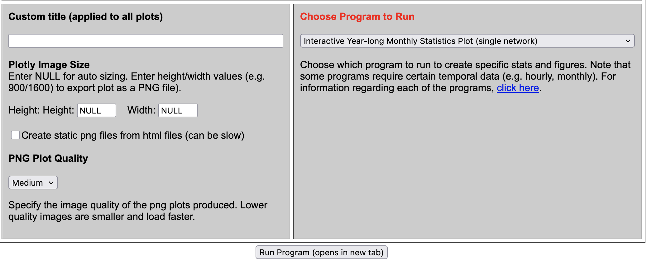
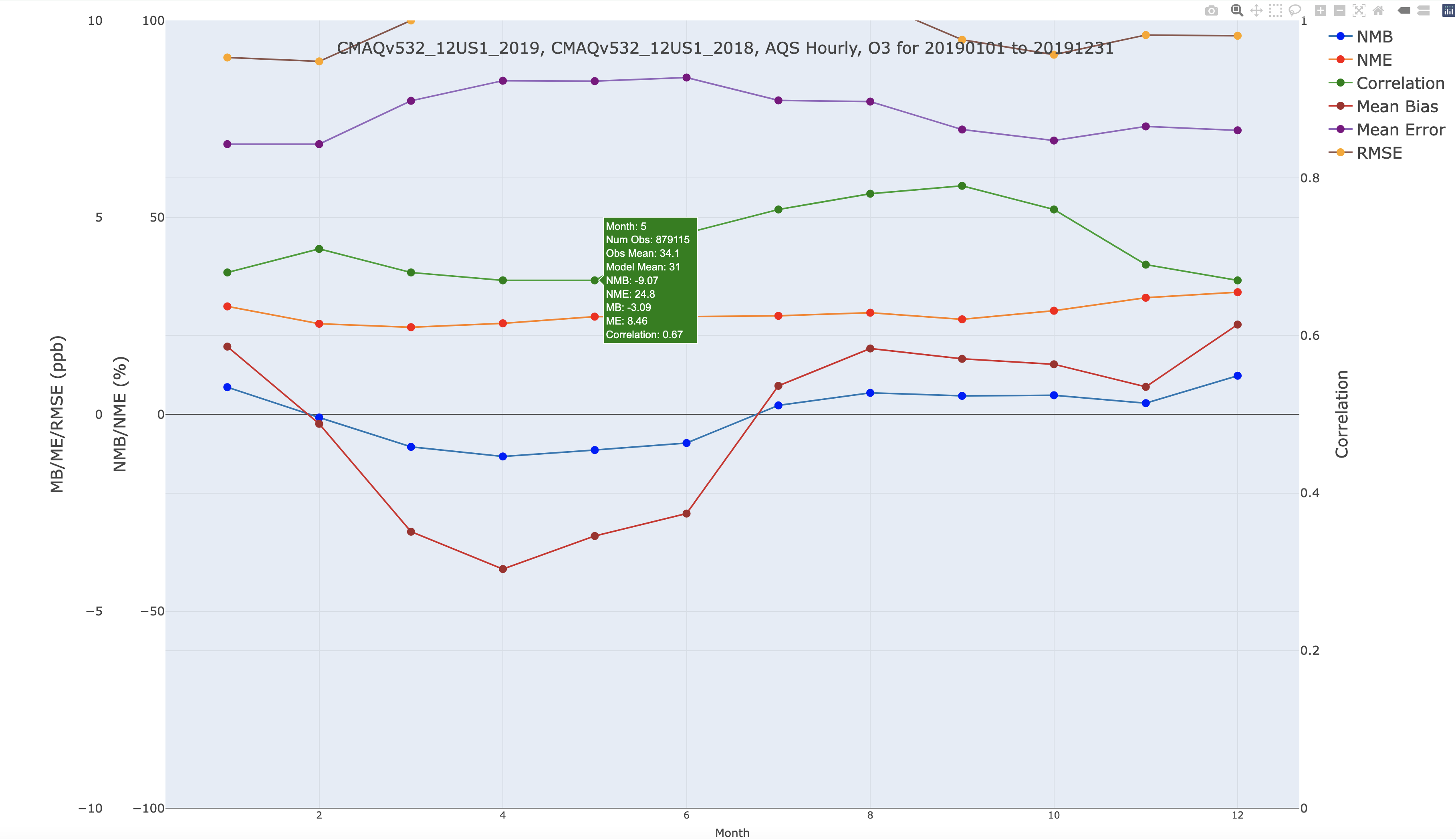
7.11.2. Create Interactive Year-long Monthly Statistics Plot (single network)

• Select Database ID
  • Select amad_EQUATES

• Select Project ID
  • Select CMAQv532_12US1_2019

• Under Observation Network
  • Select AQS Hourly

• Under Species to Plot
  • Select O3

• Under Choose Program to Run
  • Interactive Year-long Monthly Statistics Plot (single network)

Interactive Year-long Monthly Statistics Plot using Networks AQS Hourly and Ozone

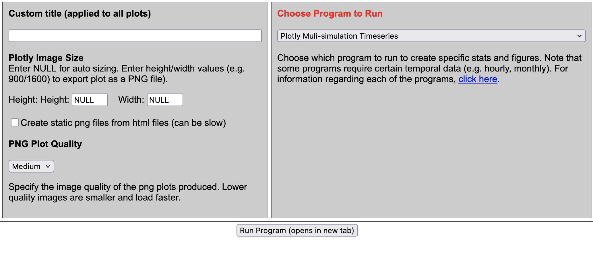
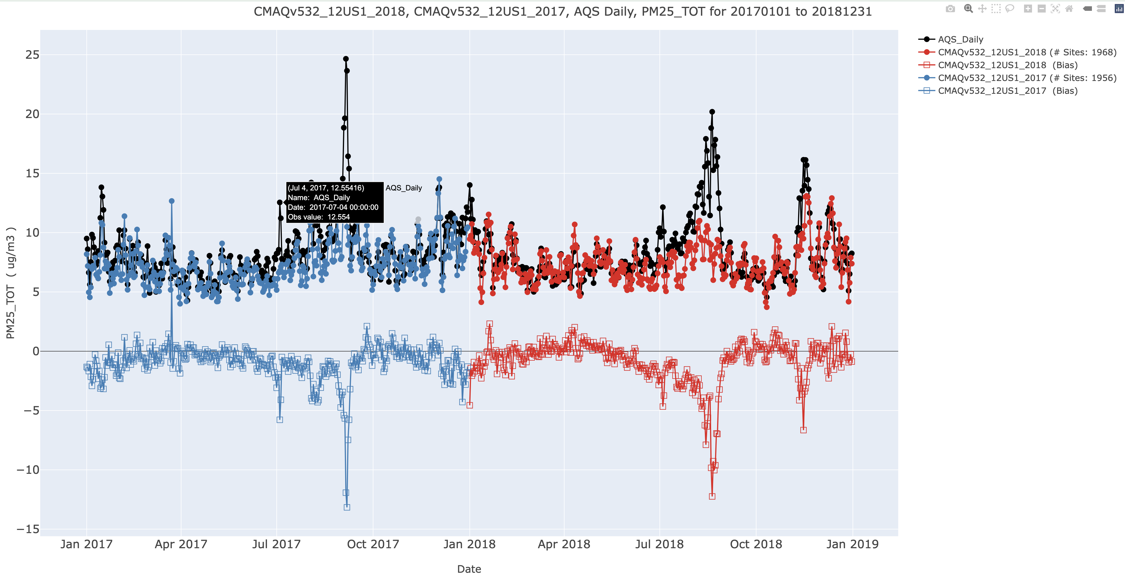
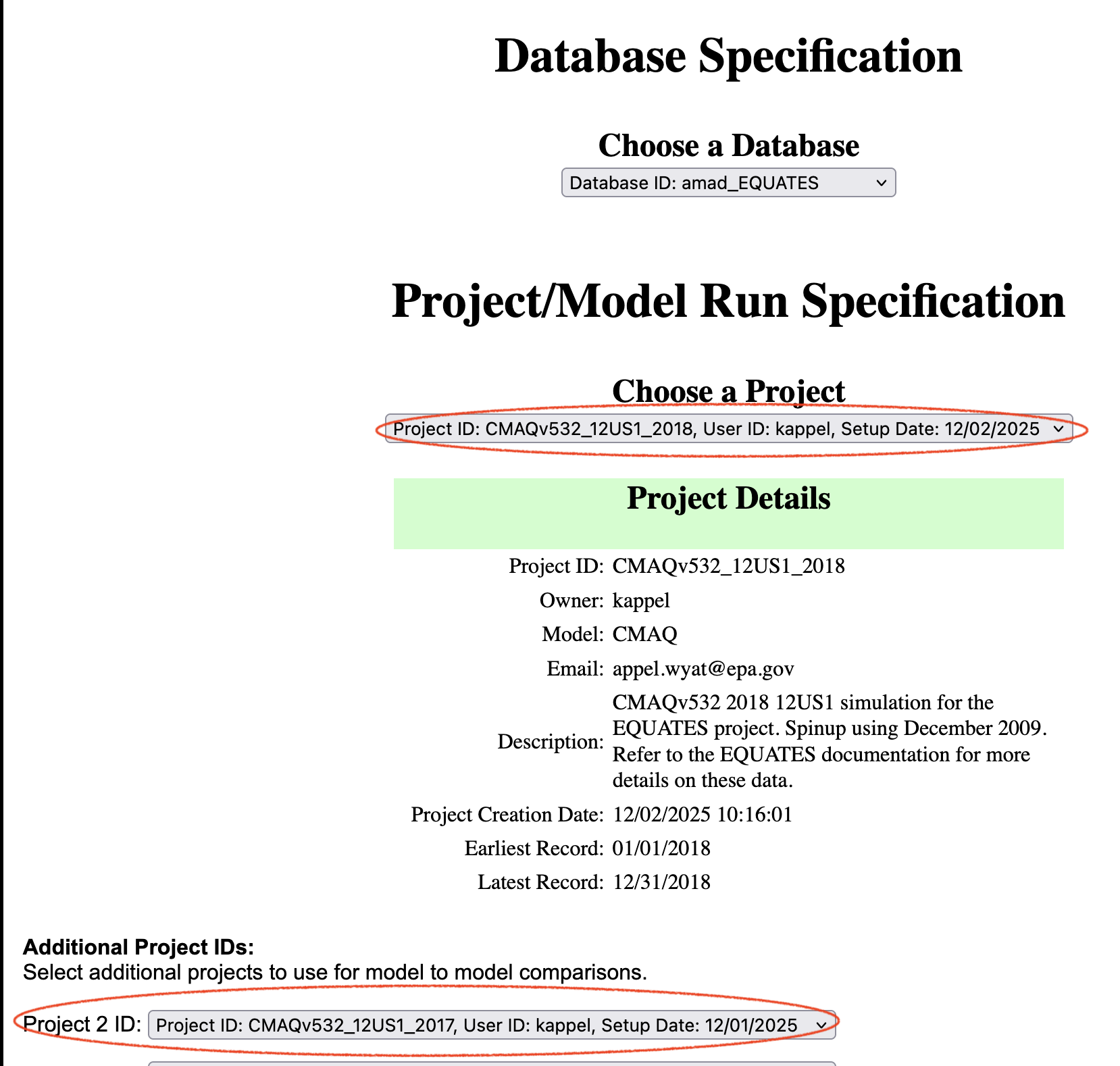
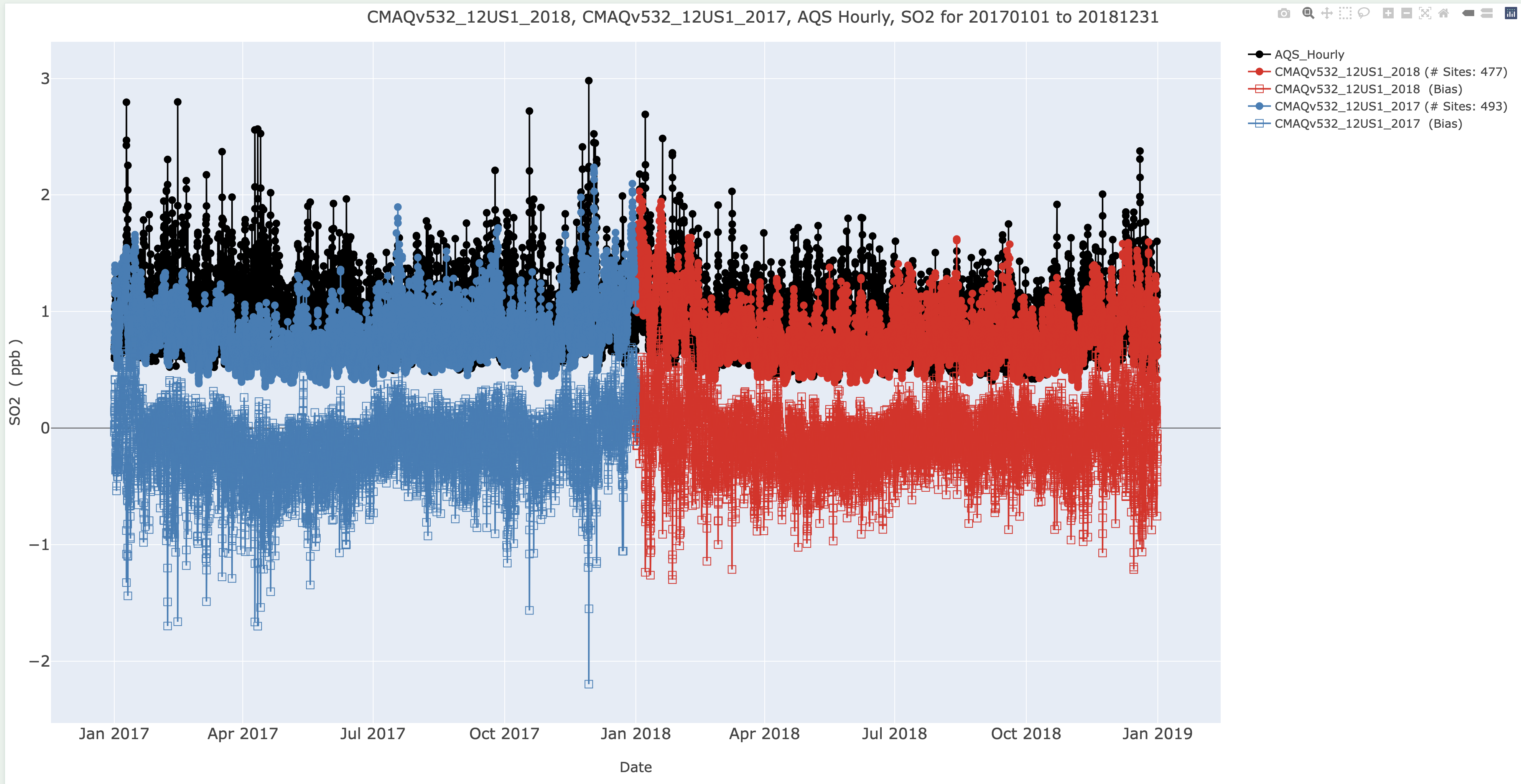
7.11.3. Create Interactive Plotly Multi-simulation Timeseries (single network)

• Select Database ID
  • Select amad_EQUATES

• Select Project ID
  • Select CMAQv532_12US1_2018
  • Select CMAQv532_12US1_2017

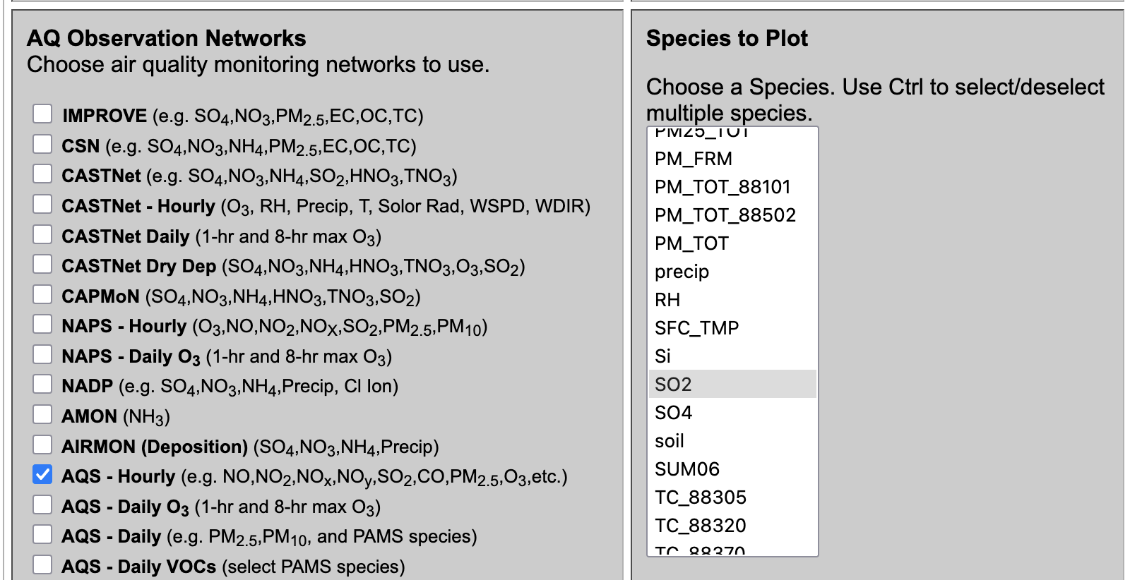
• Under Observation Network
  • Select AQS Daily (e.g. PM2.5, PM10, and PAMS species)

• Under Species to Plot
  • Select PM25_TOT

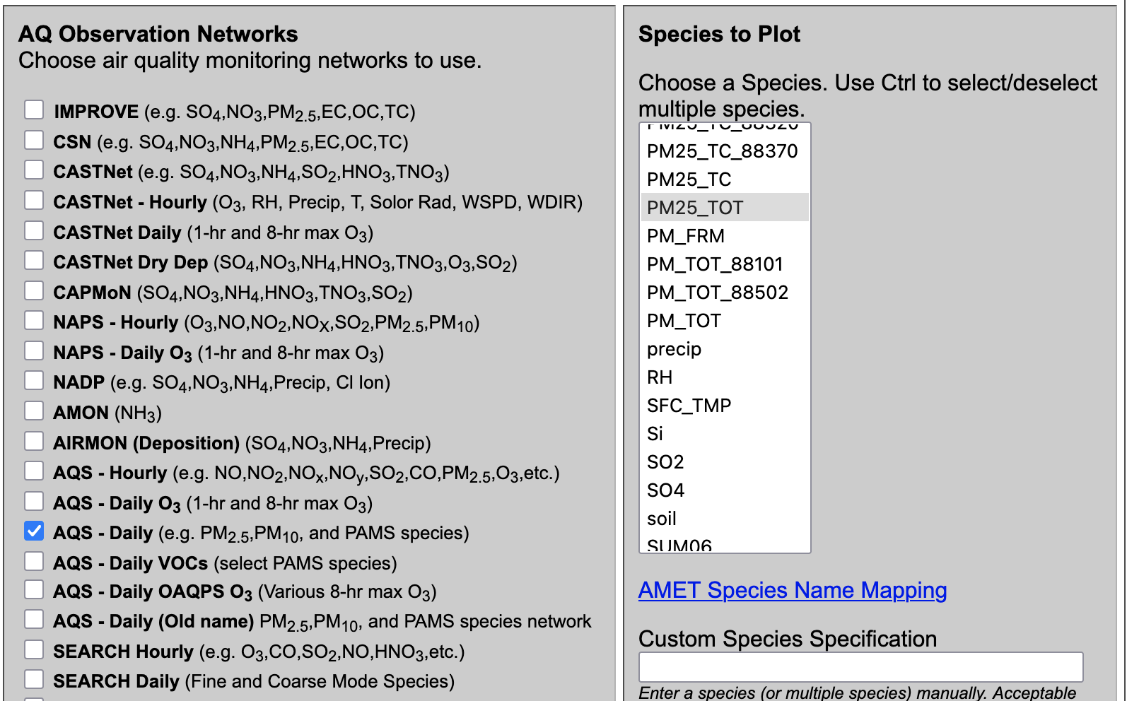
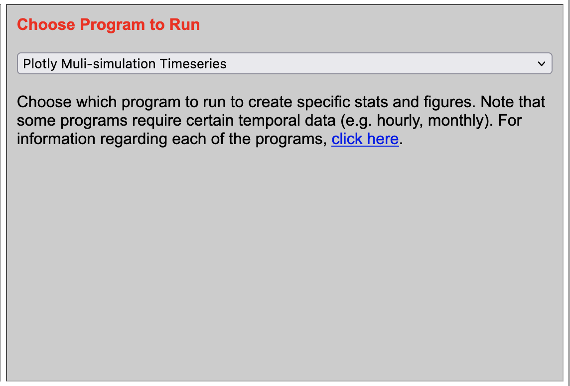
• Under Choose Program to Run
  • Plotly Multi-simulation Timeseries

Interactive Plotly Multi-simulation (EQUATES 2017, 2018) Timeseries Plot using Networks AQS Daily and PM25_TOT

7.11.4. Create Interactive Plotly Mutli-simulation Timeseries for SO2 and AQS Hourly (single network)

• Select Database ID
  • Select amad_EQUATES

• Select Project ID
  • Select CMAQv532_12US1_2018
  • Select CMAQv532_12US1_2017

• Under Observation Network
  • AQS - Hourly (e.g. NO,NO2,NOx,NOy,SO2,CO,PM2.5,O3,etc.)

• Under Species to Plot
  • Select SO2

• Under Choose Program to Run
  • Plotly Multi-simulation Timeseries

Interactive Plotly Multi-simulation (EQUATES 2017, 2018) Timeseries Plot using Networks AQS Hourly and SO2

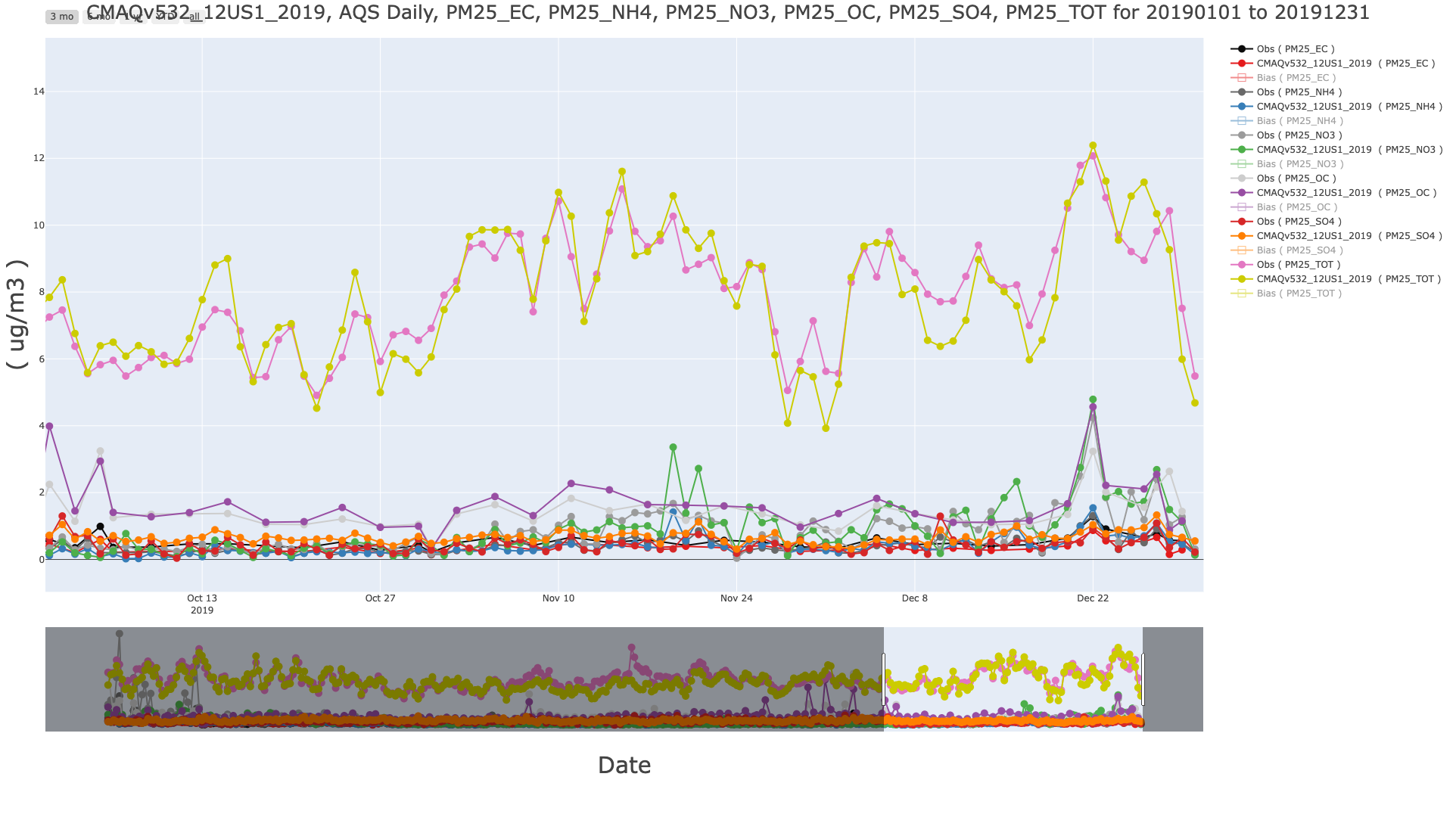
7.11.5. Create Interactive Plotly Multi-species Timeseries for PM25_TOT and major components and AQS Hourly (single network)

• Select Database ID
  • Select amad_EQUATES

• Select Project ID
  • Select CMAQv532_12US1_2019

• Under Observation Network
  • AQS - Daily (e.g. PM2.5,PM10, and PAMS species)

• Under Species to Plot
  • Select PM25_TOT, PM25_EC, PM25_NH4+, PM25_NO3, PM25_OC, PM25_SO4

• Under Choose Program to Run
  • Plotly Multi-species Timeseries

Interactive Plotly Multi-species (EQUATES 2019) Timeseries Plot using Networks AQS Daily and PM25_TOT and it's components zoomed in for 3 month period

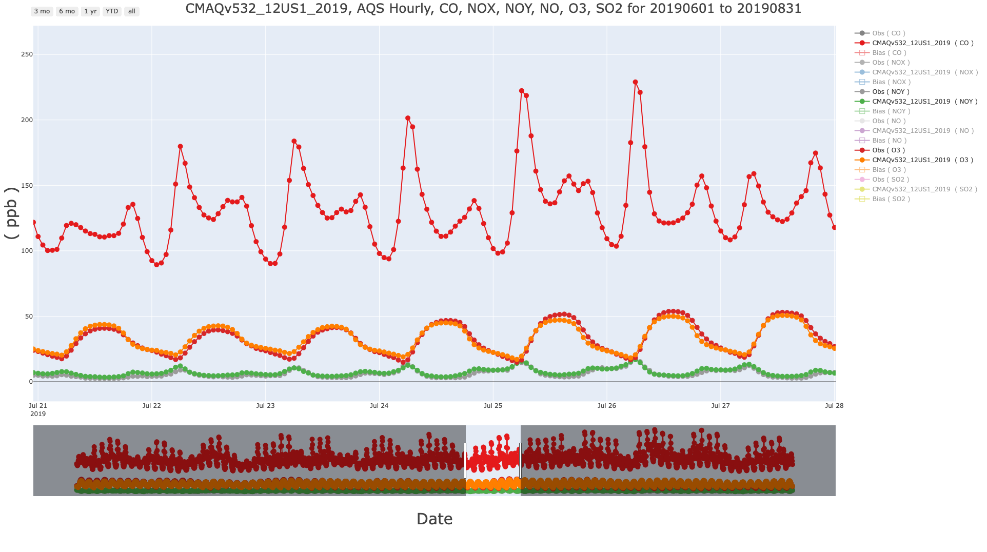
7.11.6. Create Interactive Plotly Multi-species Timeseries for O3 and Precursors and AQS Hourly (single network)

• Select Database ID
  • Select amad_EQUATES

• Select Project ID
  • Select CMAQv532_12US1_2019

• Under Observation Network
  • AQS - Hourly (e.g. NO,NO2,NOx,NOy,SO2,CO,PM2.5,O3,etc.)

• Under Species to Plot
  • Select NO,NO2,NOx,NOy,SO2,CO,PM2.5,O3

• Under Choose Program to Run
  • Plotly Multi-species Timeseries

Interactive Plotly Multi-species (EQUATES 2019) Timeseries Plot using Networks AQS Daily and it's precursors zoomed in for 3 month period

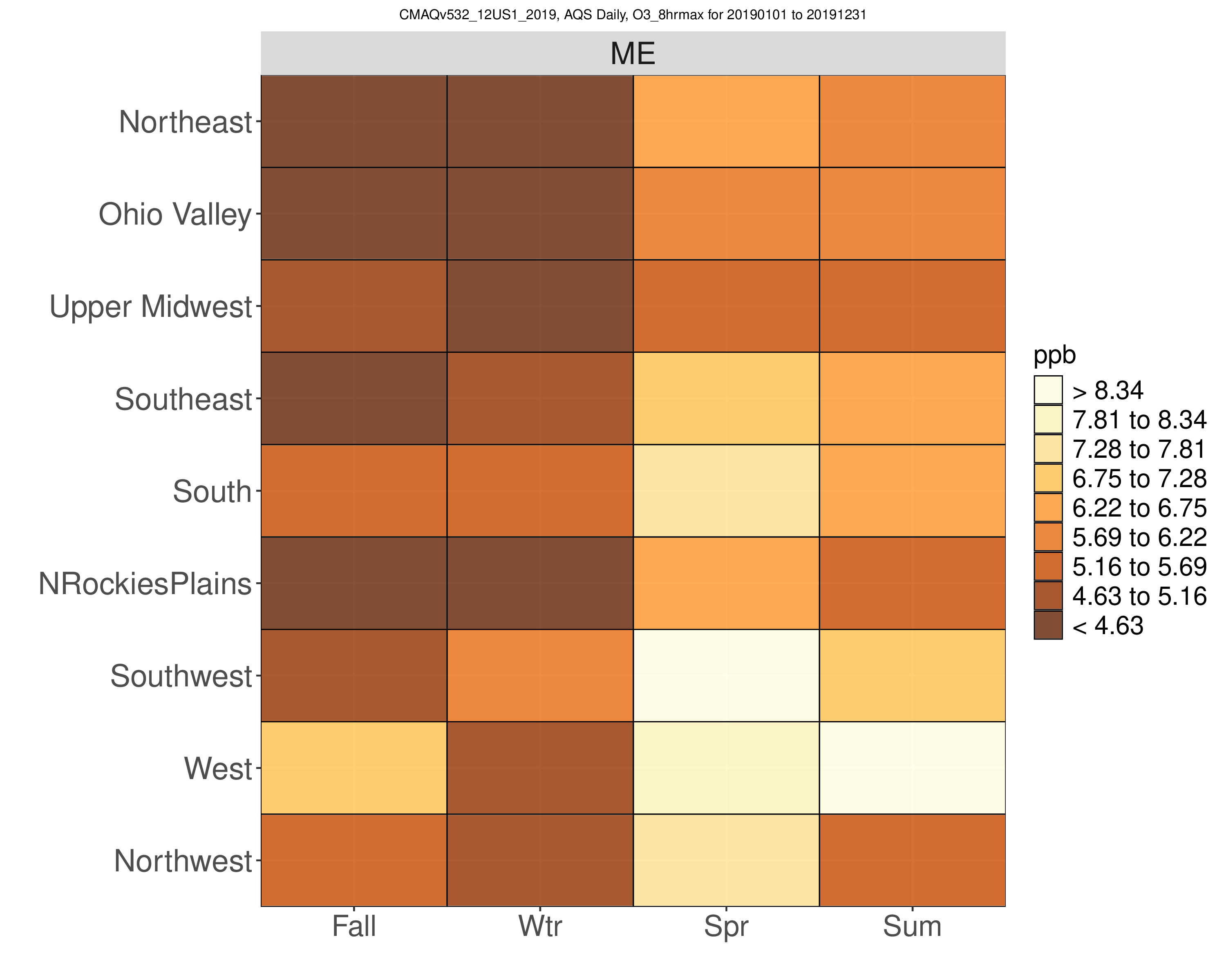
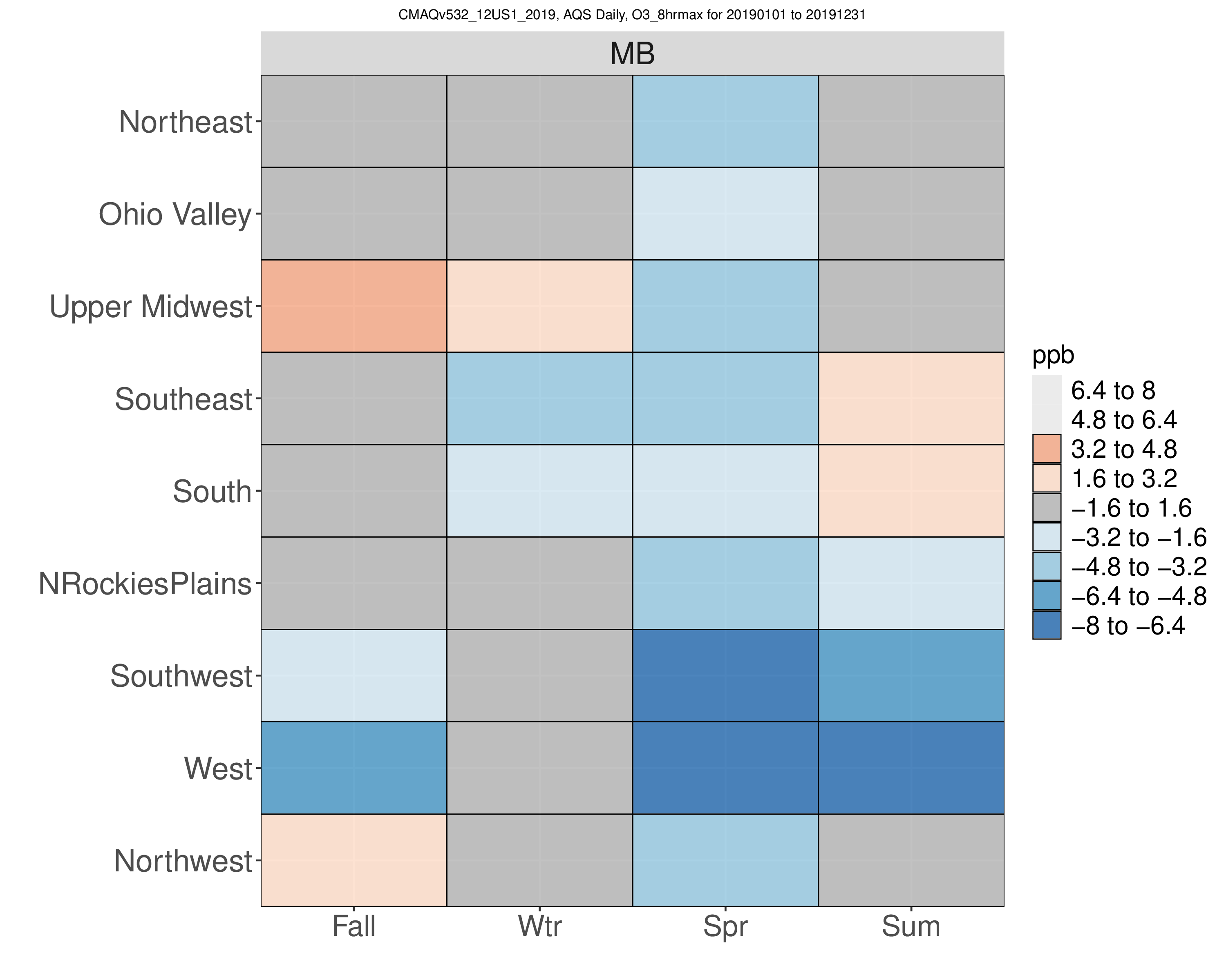
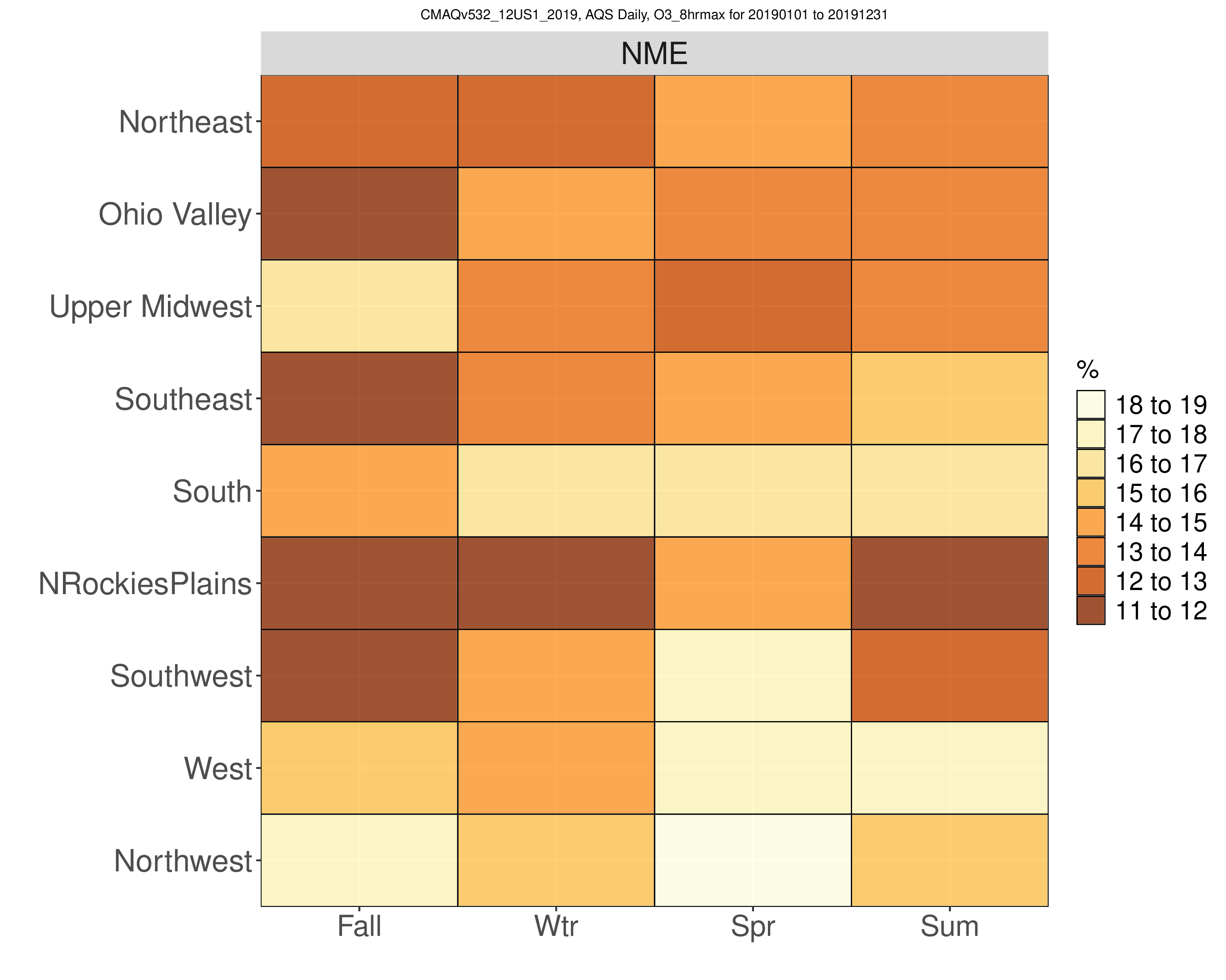
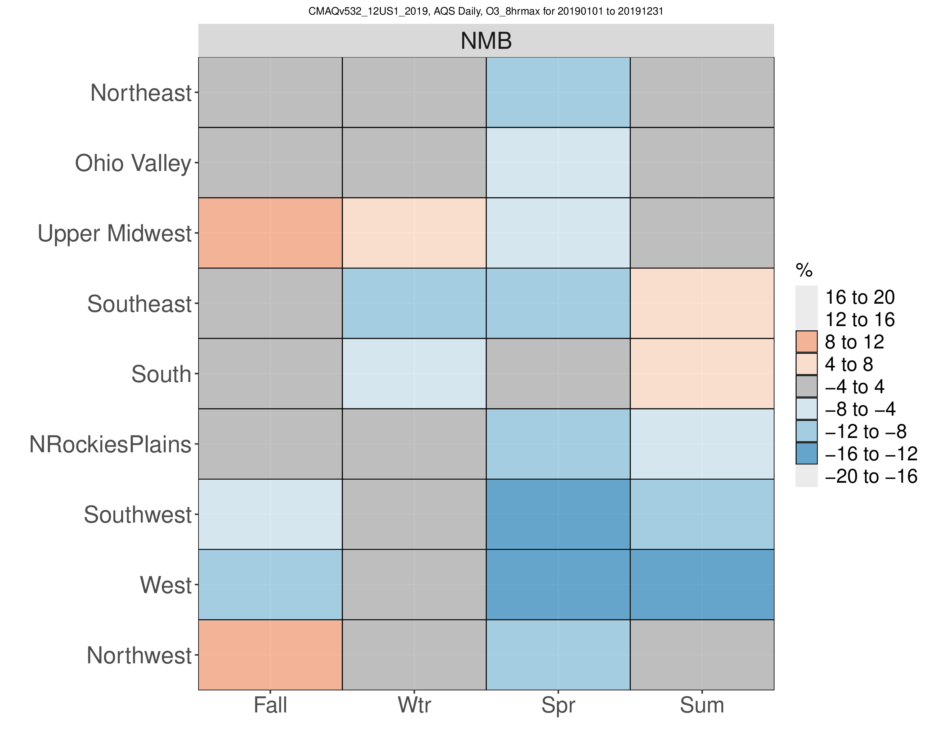
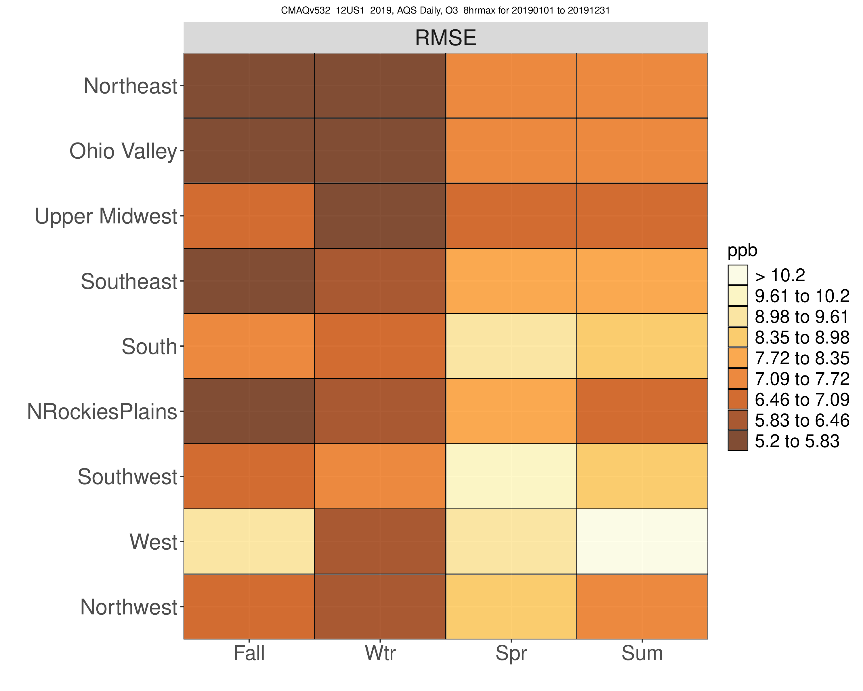
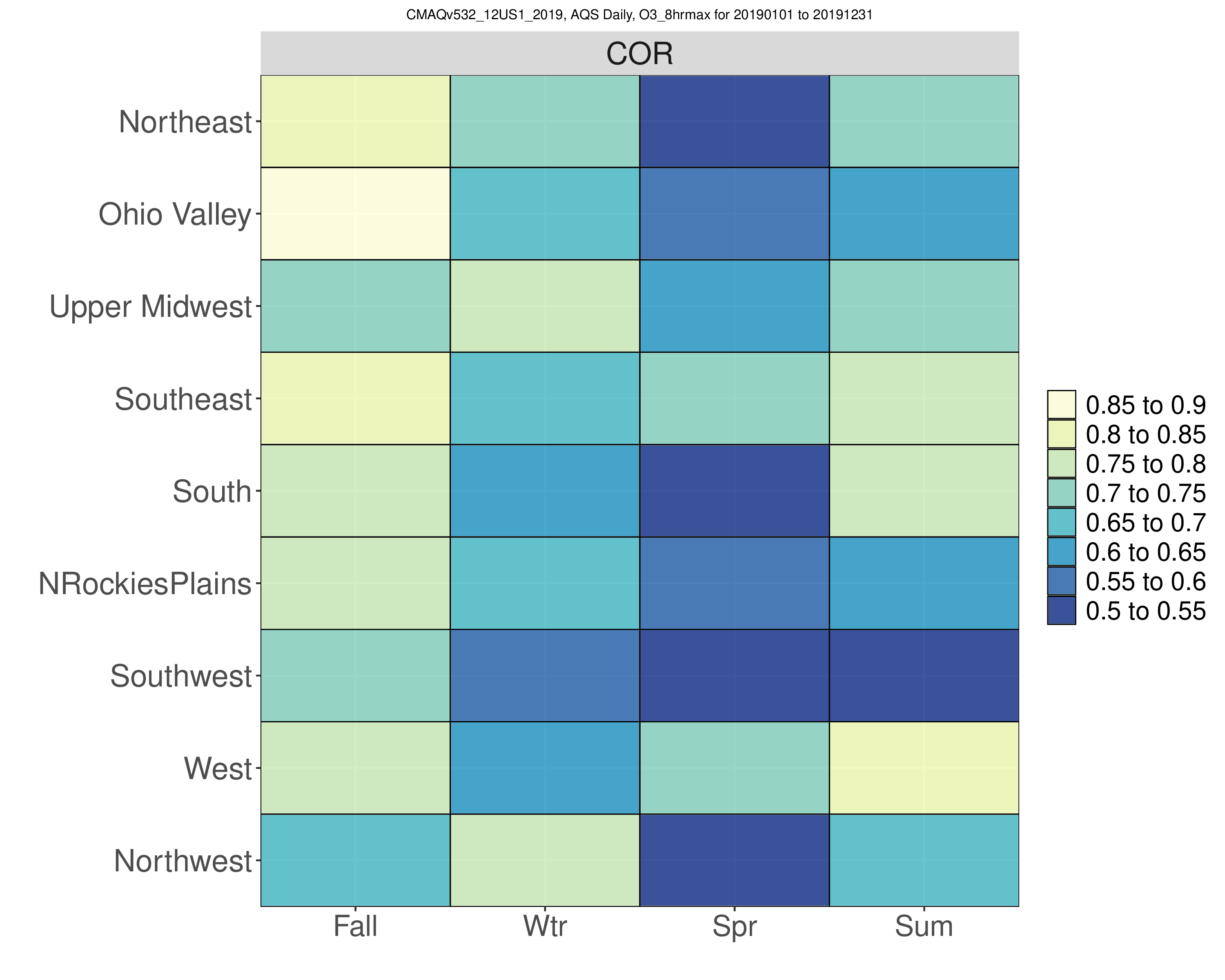
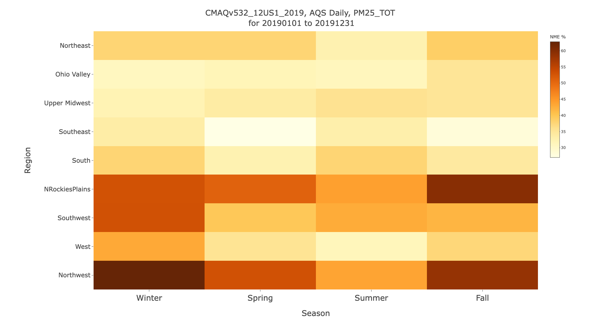
7.11.7. Create Kelly Plot (single species, single network, full year data)

• Select Database ID
  • Select amad_EQUATES

• Select Project ID
  • Select CMAQv532_12US1_2019

• Under Observation Network
  • Select AQS Daily O3 (e.g. 1-hr and 8-hr max O3))

• Under Species to Plot
  • Select O3_8hrmax

• Under Choose Program to Run
  • Kelly Plot (single species, single network, full year data)

Ozone 8hrmax Seasonal Kelly Plots

Error	Bias

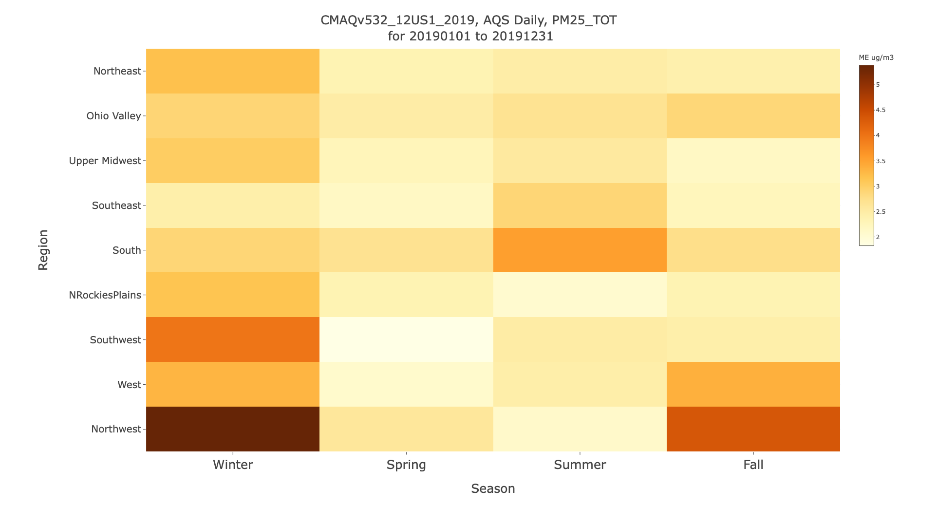
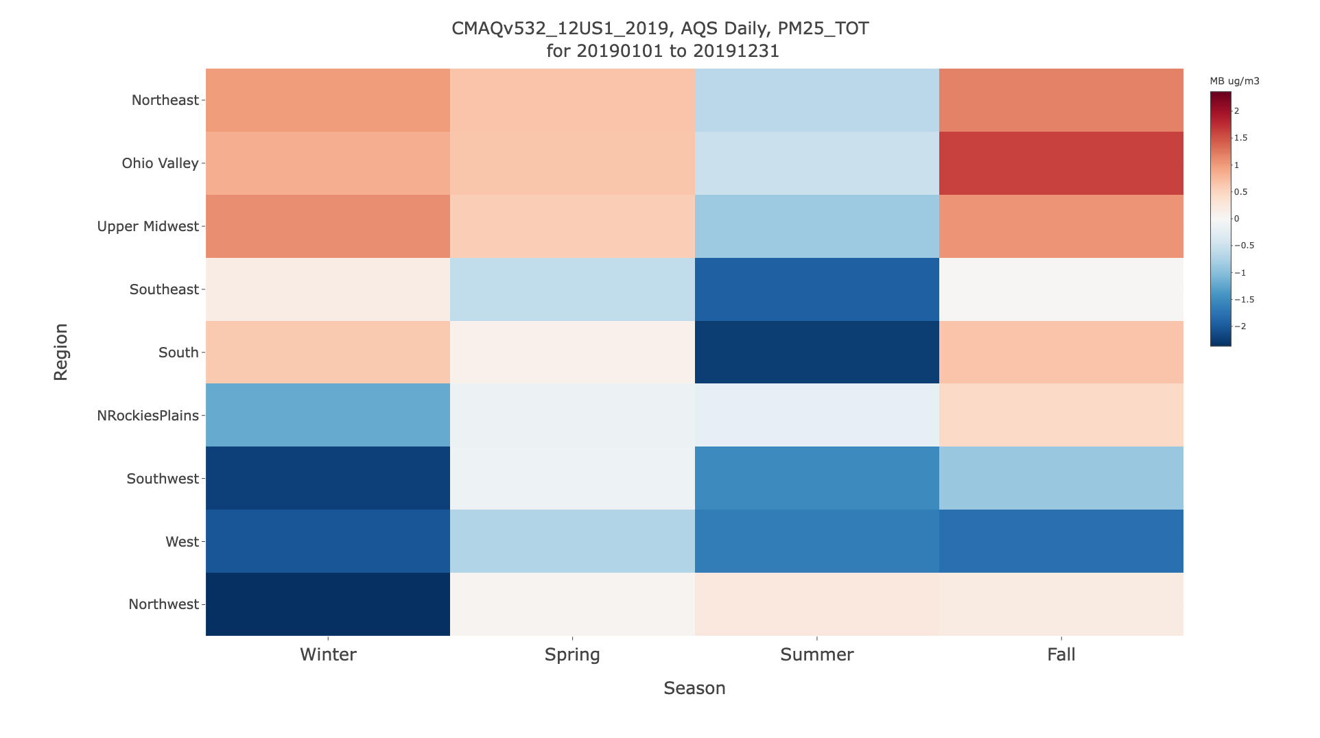
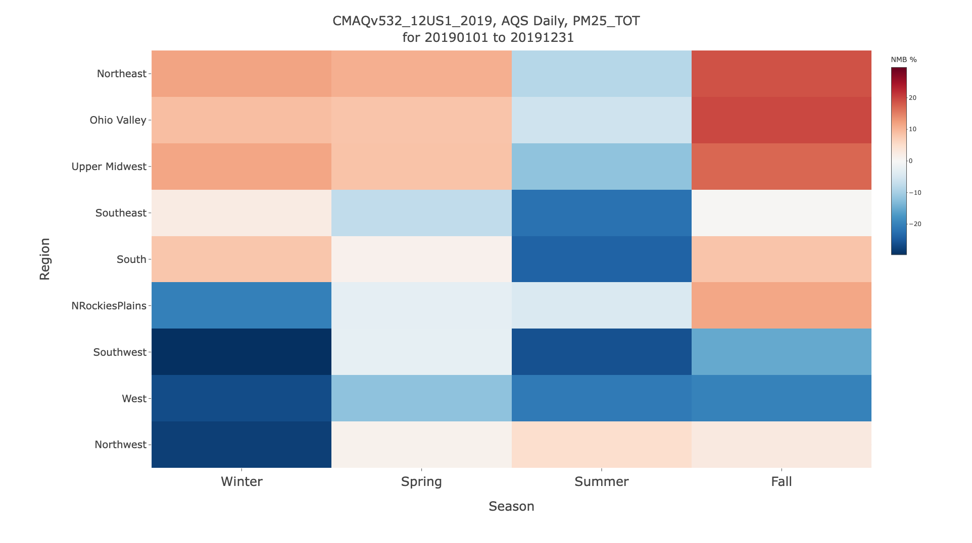
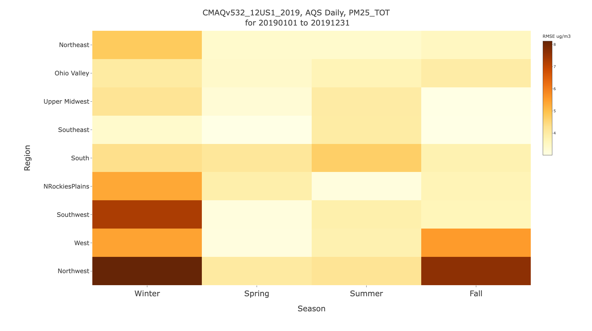
7.11.8. Create Plotly Kelly Plot (single species, single network, full year data)

• Select Database ID
  • Select amad_EQUATES

• Select Project ID
  • Select CMAQv532_12US1_2019

• Under Observation Network
  • Select AQS Daily (e.g. PM2.5,PM10, and PAMS species)

• Under Species to Plot
  • Select PM2.5_TOT

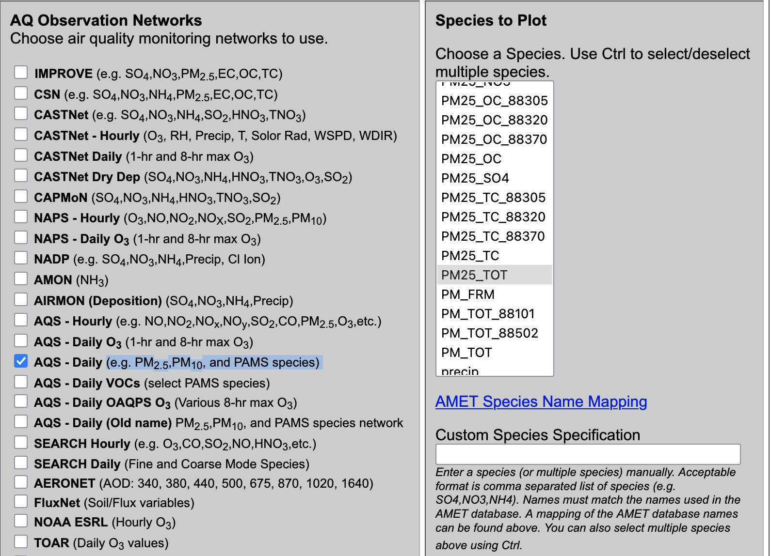
• Under Choose Program to Run
  • Plotly Kelly Plot (single species, single network, full year data)

Seasonal Daily PM2.5 Plotly Kelly Plots

Error	Bias

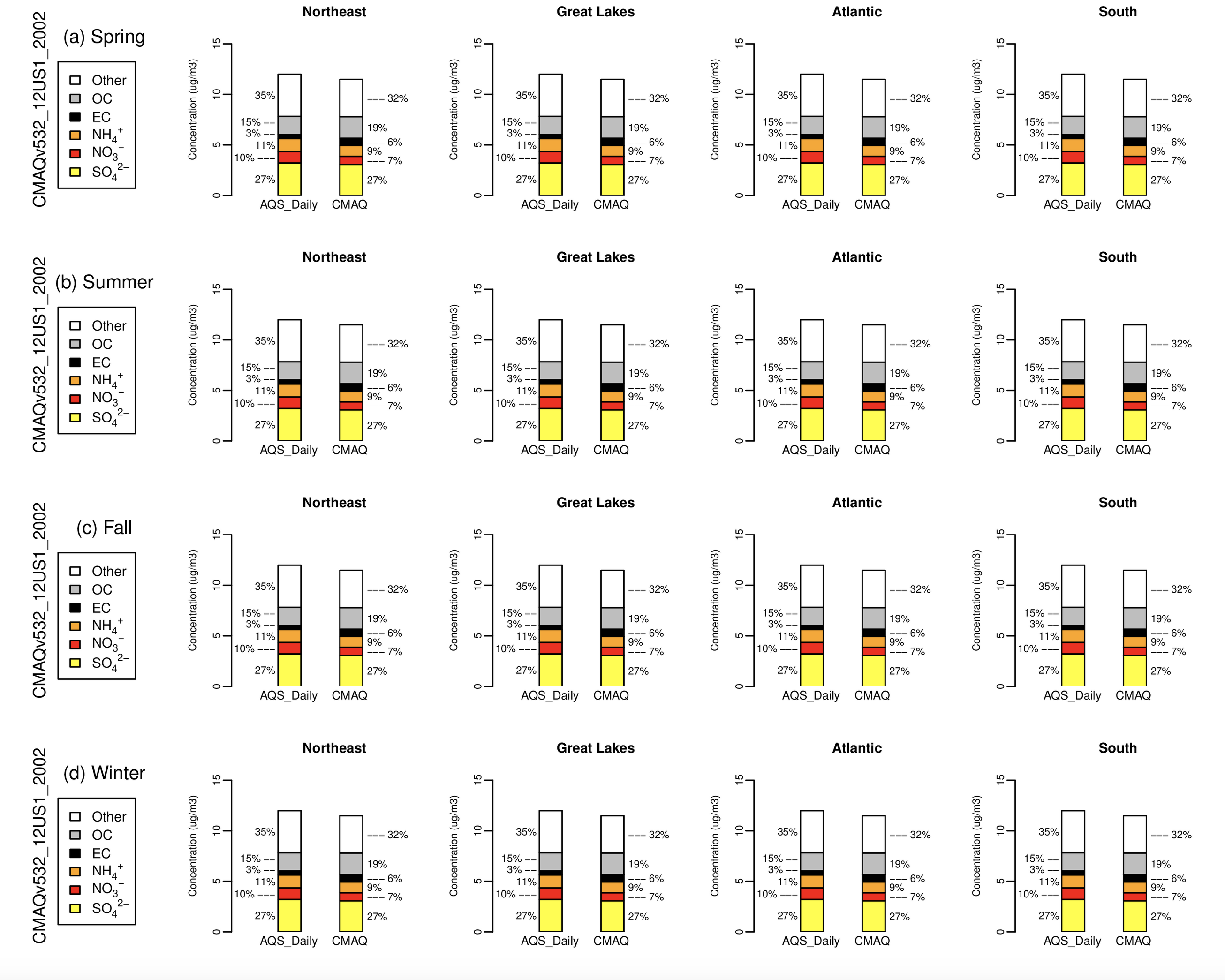
7.11.9. Create Multi-Panel Stacked Bar Plot (full year data)

• Select Database ID
  • Select amad_EQUATES

• Select Project ID
  • Select CMAQv532_12US1_2002

• Under Observation Network
  • Select AQS Daily (e.g. PM2.5,PM10, and PAMS species)

• Under Species to Plot
  • Select PM2.5_TOT

• Under Choose Program to Run
  • Multi-Panel Stacked Bar Plot AE6 (full year data)

Multi-Panel Stacked Bar Plot AQS Daily and PM2.5_TOT

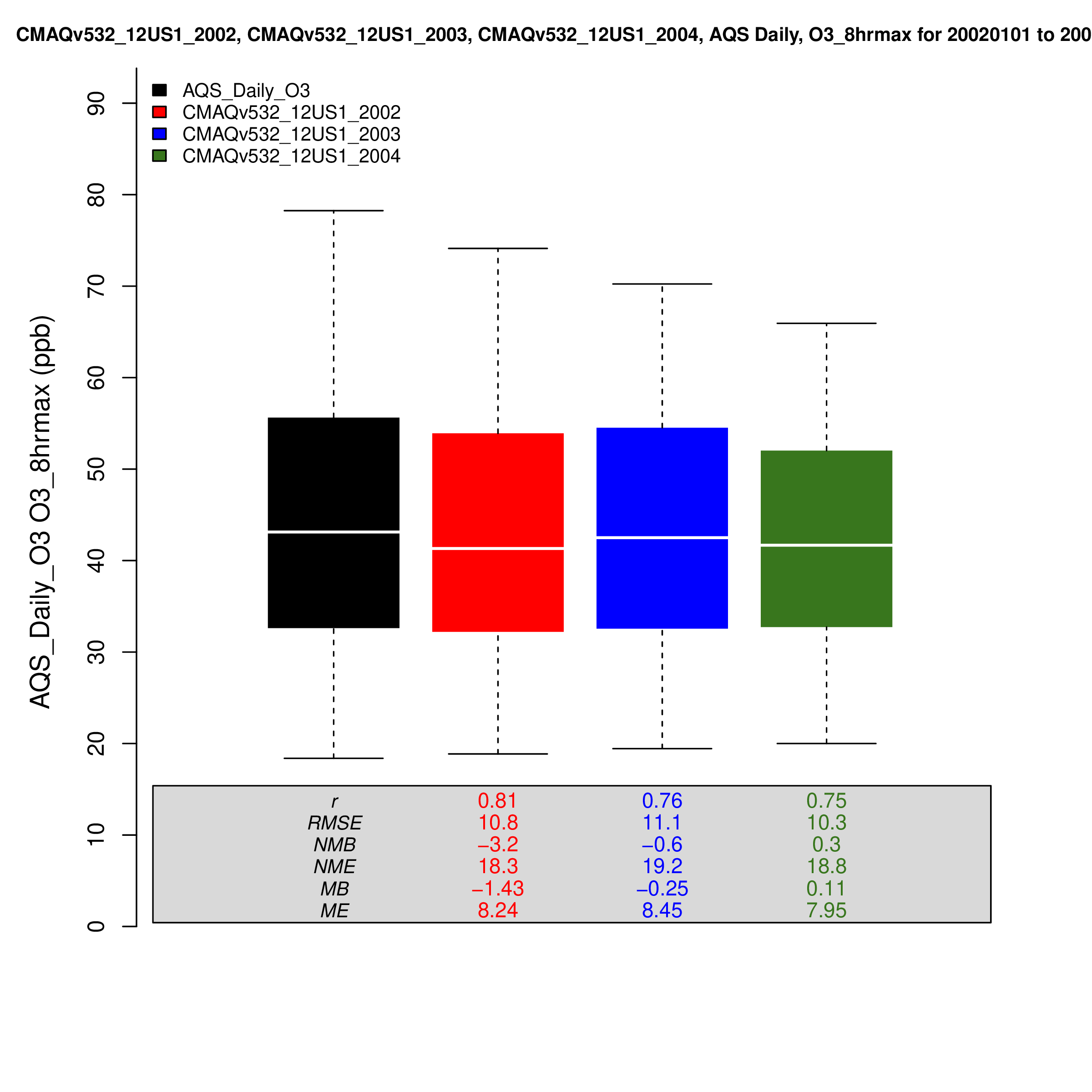
7.11.10. Create Roselle Stacked Bar Plot (full year data)

• Select Database ID
  • Select amad_EQUATES

• Select Project ID
  • Select CMAQv532_12US1_2002
  • Select CMAQv532_12US1_2003
  • Select CMAQv532_12US1_2004

• Under Observation Network
  • Select AQS Daily O3 (1-hr and 8-hr max O3)

• Under Species to Plot
  • Select O3_8hrmax

• Under Choose Program to Run
  • Roselle Boxplot

Roselle Box Plot AQS Daily O3 and O3_8hrmax for 2002-2004

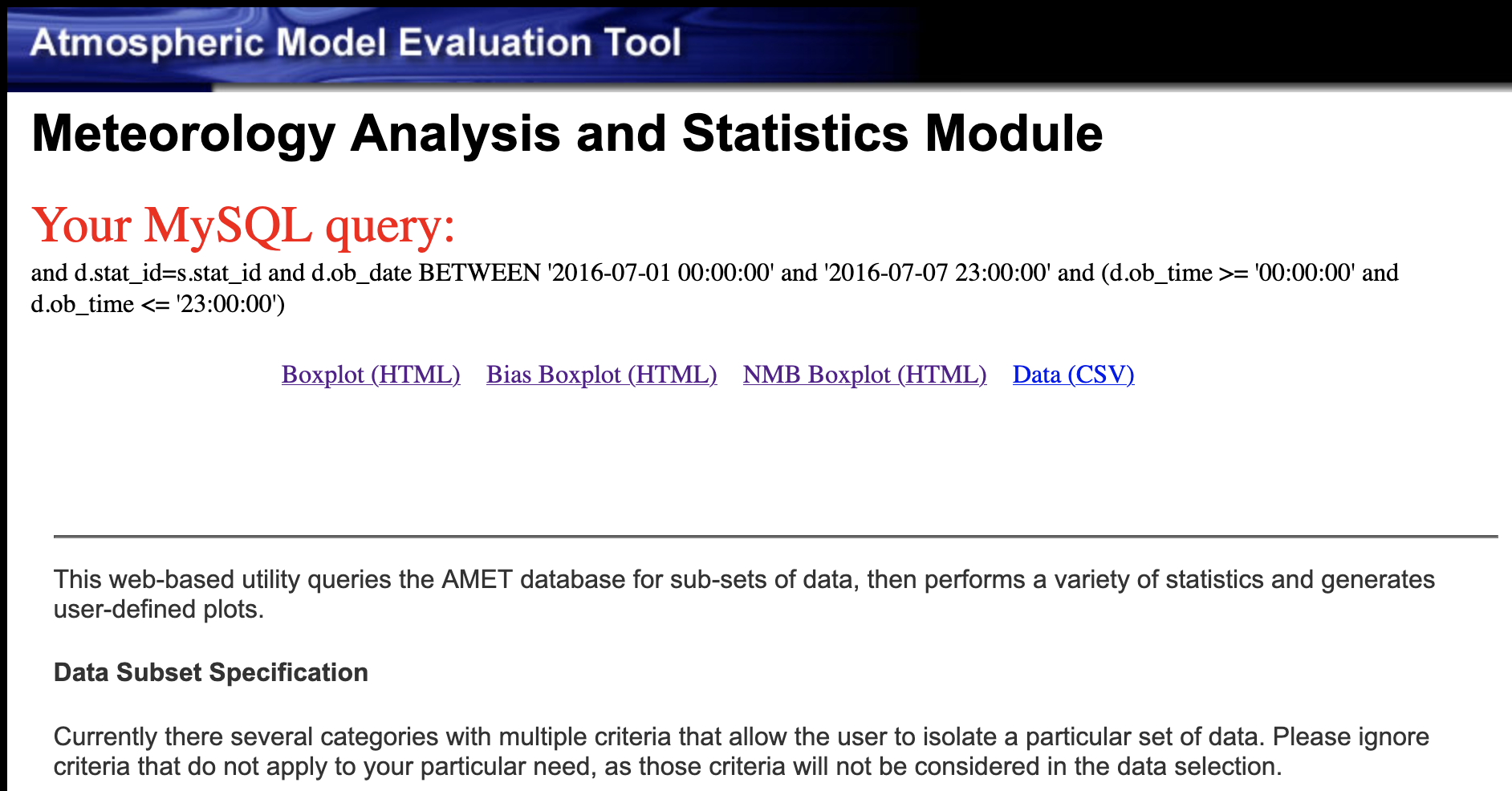
7.12. Create Met Plots using the AMET Met Website

Change the IP address to the public IP address for your instance in this example.

http://[your-ec2-external-ip-address]:443/querygen_met.php

Use the website to select the database, project, variables to plot, and plotting programs. Click on the arrow to display the list the available programs for creating different types of plots.

7.12.1. Programs to create plots

Uses can select one of 62 different programs in the AMET MET Website to create plots.

Scatter Plots (13) | Click to expand!

Name of R Script | Select Program
1. AQ_Scatterplot.R | Multiple Networks Model/Ob Scatterplot (select stats only)
2. AQ_Scatterplot_ggplot.R | GGPlot Scatterplot (multi network, single run)
3. AQ_Scatterplot_plotly.R | Interactive Multiple Network Scatterplot
4. AQ_Scatterplot_multisim_plotly.R | Interactive Multiple Simulation Scatterplot
5. AQ_Scatterplot_single.R | Single Network Model/Ob Scatterplot (includes all stats)
6. AQ_Scatterplot_density.R | Density Scatterplot (single run, single network)
7. AQ_Scatterplot_density_ggplot.R | GGPlot Density Scatterplot (single run, single network)
8. AQ_Scatterplot_mtom.R | Model/Model Scatterplot (multiple networks)
9. AQ_Scatterplot_mtom_density_ggplot.R | Model/Model Density Scatterplot (single network)
10. AQ_Scatterplot_percentiles.R | Scatterplot of Percentiles (single network, single run)
11. AQ_Scatterplot_bins.R | Binned MB & RMSE Scatterplots (single net., mult. run)
12. AQ_Scatterplot_bins_plotly.R | nteractive Binned Plot (single net., mult. run)
13. AQ_Scatterplot_multi.R | Multi Simulation Scatter plot (single network, mult runs)

Timeseries Plots (12) | Click to expand!

Name of R Script | Program
1. AQ_Timeseries.R | Time-series Plot (single network, multiple sites averaged)
2. AQ_Timeseries_bysite.R | Individual Site Time-series Plots (single network, multiple sites not average)
3. AQ_Timeseries_dygraph.R | Dygraph Time-series Plot (single network, multiple sites averaged)
4. AQ_Timeseries_plotly.R | Plotly Muli-simulation Timeseries
5. AQ_Timeseries_plotly_bysite.R | Individual Site Plotly Time-series Plots (single network, multiple sites not average)
6. AQ_Timeseries_networks_plotly.R | Plotly Multi-network Timeseries
7. AQ_Timeseries_species_plotly.R | Plotly Multi-species Timeseries
8. AQ_Timeseries_multi_networks.R | Multi-Network Time-series Plot (mult. net., single run)
9. AQ_Timeseries_multi_species.R | Multi-Species Time-series Plot (mult. species, single run)
10. AQ_Timeseries_MtoM.R | Model-to-Model Time-series Plot (single net., multi run)
11. AQ_Monthly_Stat_Plot.R | Year-long Monthly Statistics Plot (single network)
12. AQ_Monthly_Stat_Plot_plotly.R | Interactive Year-long Monthly Statistics Plot (single network)

Spatial Plots (13) | Click to expand!

Name of R Script | Program
1. AQ_Stats_Plots.R | Species Statistics and Spatial Plots (multi networks)
2. AQ_Stats_Plots_leaflet.R | Interactive Species Statistics and Spatial Plots (single plot)
3. AQ_Stats_Plots_leaflet_network.R | Interactive Species Statistics and Spatial Plots (multiple plots)
4. AQ_Plot_Spatial.R | Spatial Plot (multi networks)
5. AQ_Plot_Spatial_leaflet.R | Interactive Spatial Plot
6. AQ_Plot_Spatial_leaflet_network.R | Interactive Spatial Plot (multiple plots)
7. AQ_Plot_Spatial_Species_Diff_leaflet.R | Interactive Species Diff Spatial Plot (multi networks,multi species)
8. AQ_Plot_Spatial_MtoM.R | Model/Model Diff Spatial Plot (multi network, multi run)
9. AQ_Plot_Spatial_MtoM_leaflet.R | Interactive Model/Model Diff Spatial Plot (multi network, multi run)
10. AQ_Plot_Spatial_MtoM_Species.R | Model/Model Species Diff Spatial Plot (multi network, multi run)
11. AQ_Plot_Spatial_Diff.R | Spatial Plot of Bias/Error Difference (multi network, multi run)
12. AQ_Plot_Spatial_Diff_leaflet.R | Interactive Spatial Plot of Bias/Error Difference (single plot)
13. AQ_Plot_Spatial_Diff_leaflet_network.R | Interactive Spatial Plot of Bias/Error Difference (multiple plots)

Box Plots (7) | Click to expand!

Name of R Script | Program
1. AQ_Boxplot.R | Boxplot (single network, multi run)
2. AQ_Boxplot_ggplot.R | GGPlot Boxplot (single network, multi run)
3. AQ_Boxplot_plotly.R | Plotly Boxplot (single network, multi run)
4. AQ_Boxplot_DofW.R | Day of Week Boxplot (single network, multiple runs)
5. AQ_Boxplot_Hourly.R | Hourly Boxplot (single network, multiple runs)
6. AQ_Boxplot_MDA8.R | 8hr Average Boxplot (single network, hourly data, can be slow)
7. AQ_Boxplot_Roselle.R | Roselle Boxplot (single network, multiple simulations)

Misc Plots (14) | Click to expand!

Name of R Script | Program
1. AQ_Kellyplot.R | Kelly Plot (single species, single network, full year data)
2. AQ_Kellyplot_plotly.R | Plotly Kelly Plot (single species, single network, full year data)
3. AQ_Kellyplot_region.R | Climate Region Kelly Plot (single species, single network, multi sim)
4. AQ_Kellyplot_region_plotly.R | Plolty Climate Region Kelly Plot (single species, single network, multi sim)
5. AQ_Kellyplot_season.R | Seasonal Kelly Plot (single species, single network, multi sim)
6. AQ_Kellyplot_season_plotly.R | Plotly Seasonal Kelly Plot (single species, single network, multi sim)
7. AQ_Stats.R | Species Statistics (multi species, single network)
8. AQ_Raw_Data.R | Create raw data csv file (single network, single simulation)
9. AQ_Soccerplot.R | Soccergoal" plot (multiple networks)
10. AQ_Soccerplot_plotly.R | Plotly "Soccergoal" plot (multiple networks/species)
11. AQ_Bugleplot.R | "Bugle" plot (multiple networks)
12. AQ_Histogram.R | Histogram (single network/species only)
13. AQ_Histogram_plotly.R | Interactive Histogram (single network, single species, multi run)
14. AQ_Temporal_Plots.R | CDF, Q-Q, Taylor Plots (single network, multi run)

Experimental Scripts (3) | Click to expand!

Name of R Script | Program (may not work correctly)
1. AQ_Overlay_File.R | Create PAVE/VERDI Obs Overlay File (hourly/daily data only)
2. AQ_Scatterplot_log.R | Log-Log Model/Ob Scatterplot (multiple networks)
3. AQ_Spectral_Analysis.R | Spectral Analysis (single network, single run, experimental)

7.13. Met Observation Networks

Available Meteorology Observation Networks | Click to expand!

Meteorology Network (select METAR, not sure about other networks)
1. All
2. METAR
3. AIRNOW
4. ASOS
5. Maritime
6. SAO
7. Other-Mtr

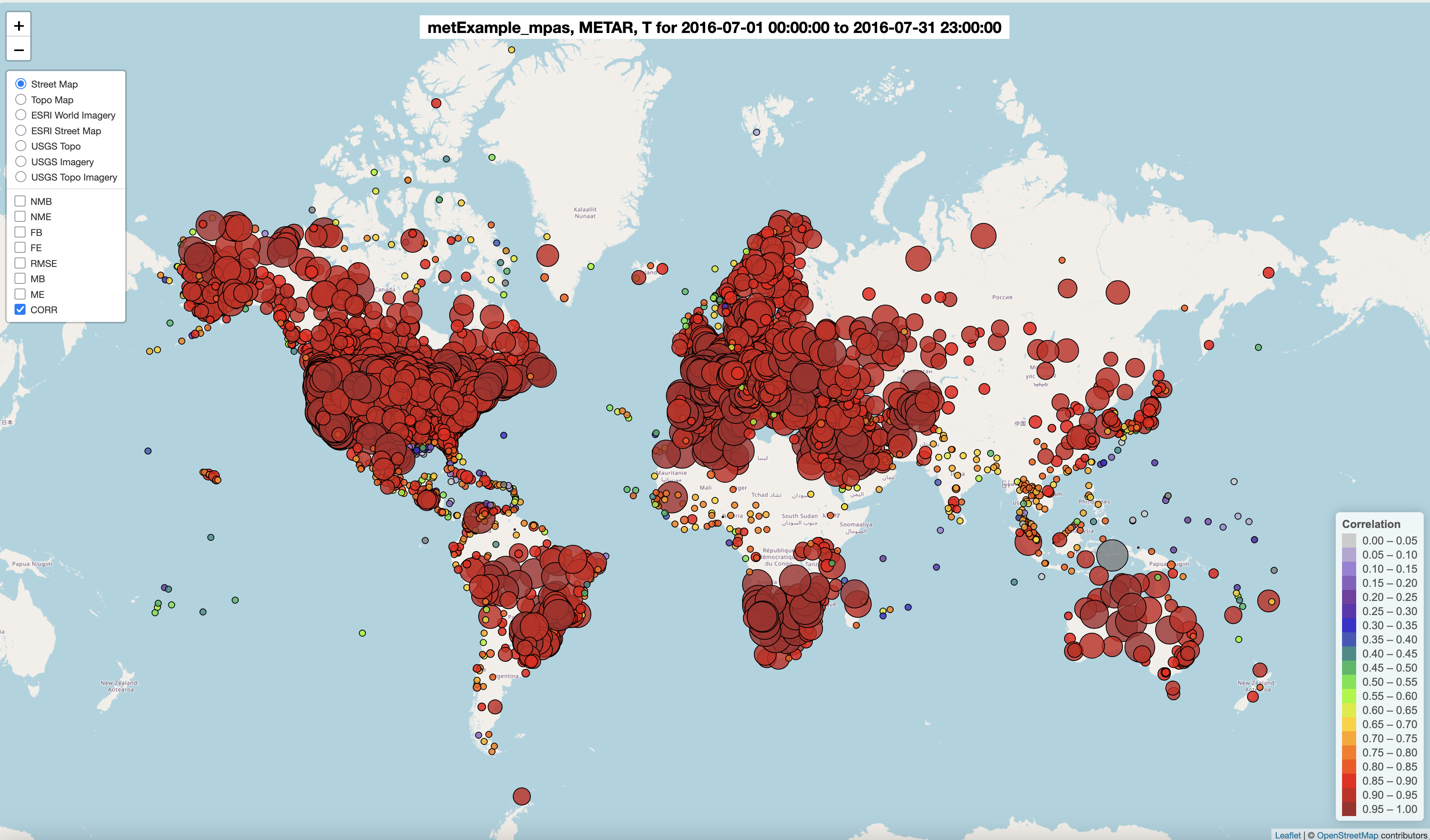
Currently, AMET_Webite supports only T2 (2 meter Temperature) from the METAR Observation Network

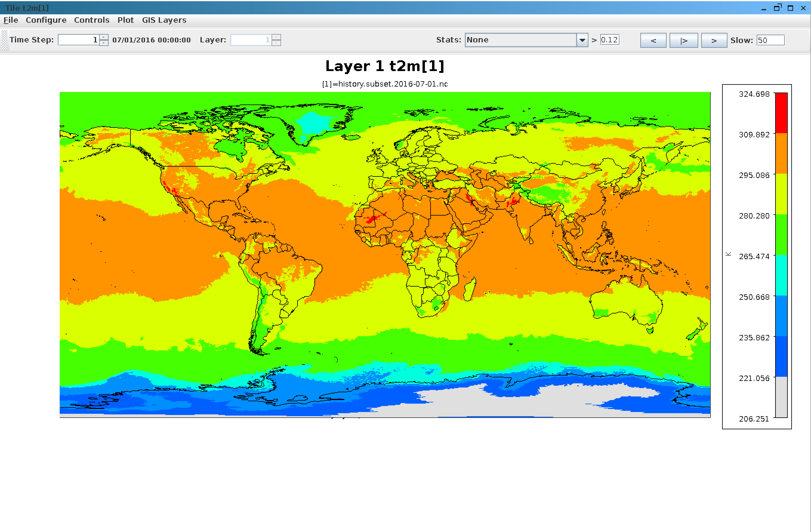
7.13.1. Map of World METAR Stations

Link to AMET User Guide World METAR Map of Temperature

Projects | Click to expand!

aqExample Grid Details
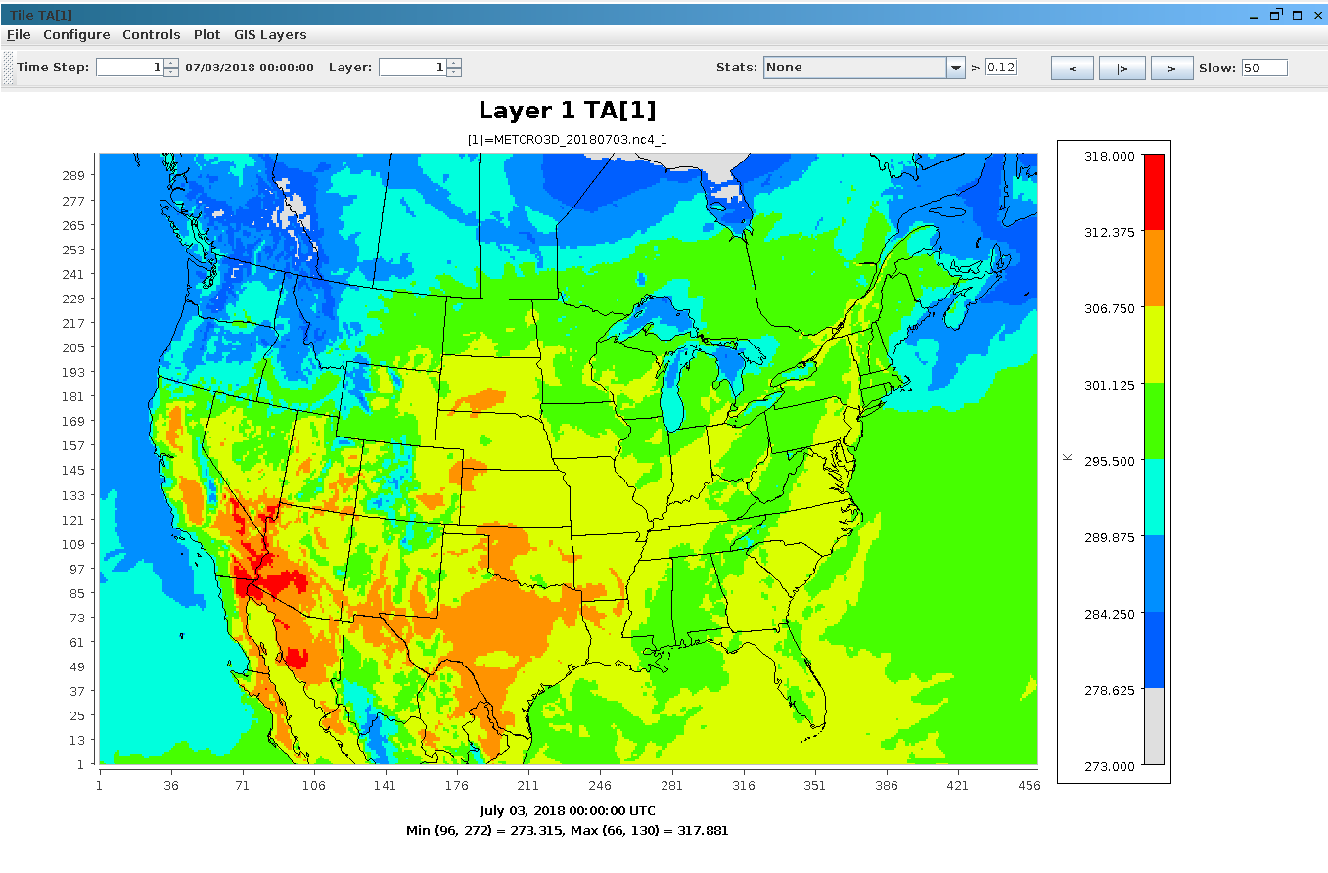
1. metExample_mcip
2. // global attributes:
3. :IOAPI_VERSION = "ioapi-3.2: $Id: init3.F90 1 2017-06-10 18:05:20Z coats $ " ;
4. :EXEC_ID = "mcip " ;
5. :FTYPE = 1 ;
6. :CDATE = 2022102;
7. :CTIME = 185908 ;
8. :WDATE = 2022102 ;
9. :WTIME = 185908 ;
10. :SDATE = 2018184 ;
11. :STIME = 0 ;
12. :TSTEP = 10000 ;
13. :NTHIK = 1 ;
14. :NCOLS = 459 ;
15. :NROWS = 299 ;
16. :NLAYS = 1 ;
17. :NVARS = 41 ;
18. :GDTYP = 2 ;
19. :P_ALP = 33. ;
20. :P_BET = 45. ;
21. :P_GAM = -97. ;
22. :XCENT = -97. ;
23. :YCENT = 40. ;
24. :XORIG = -2556000. ;
25. :YORIG = -1728000. ;
26. :XCELL = 12000. ;
27. :YCELL = 12000. ;

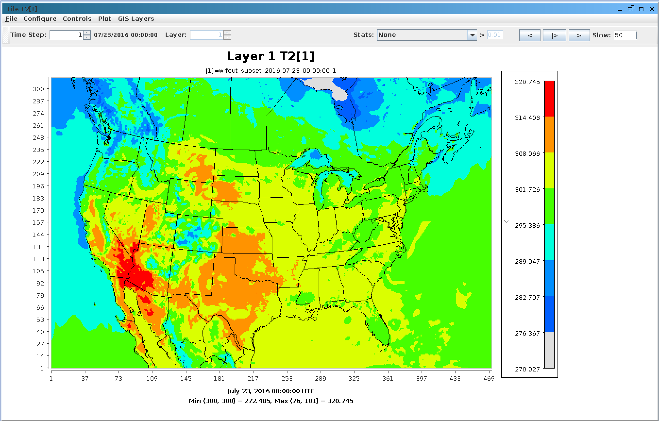
metExample_wrf Grid Details
1. // global attributes:
2. :TITLE = " OUTPUT FROM WRF V3.8 MODEL" ;
3. :START_DATE = "2016-06-29_00:00:00" ;
4. :SIMULATION_START_DATE = "2015-12-21_00:00:00" ;
5. :WEST-EAST_GRID_DIMENSION = 472 ;
6. :SOUTH-NORTH_GRID_DIMENSION = 312 ;
7. :BOTTOM-TOP_GRID_DIMENSION = 36 ;
8. :DX = 12000.f ;
9. :DY = 12000.f ;

VERDI Plot of TA in METCRO3D_20180703.nc4

metExample_wrf

VERDI Plot of T2 in wrfout

VERDI Plot of T2 in metExample_mpas

More details about understanding WRF Output data
WRF Output Description

More details about MPAS Atmosphere
MPAS Atmosphere

More details about MPAS-CMAQ
MPAS-CMAQ Model

7.13.2. Create 2m Temperature Spatial Plots

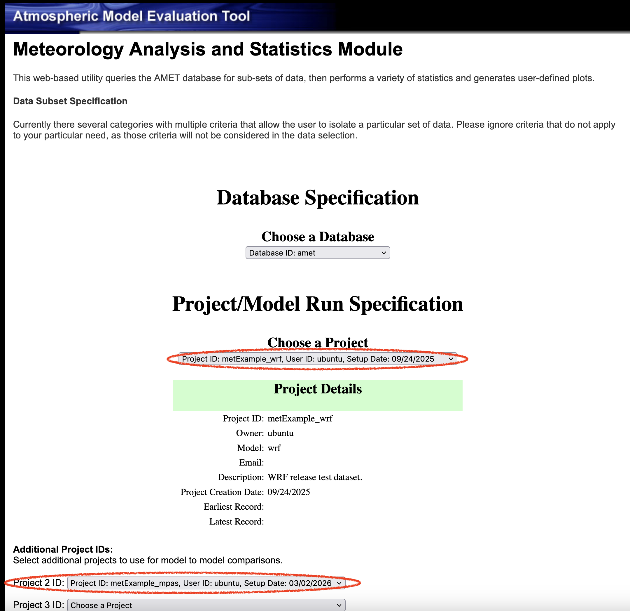
• Choose database
  • select amet
• Choose project 1
  • MetExample_wrf
• Choose project 2
  • MetExample_mpas

• Choose Met Species
  • select T(2m)

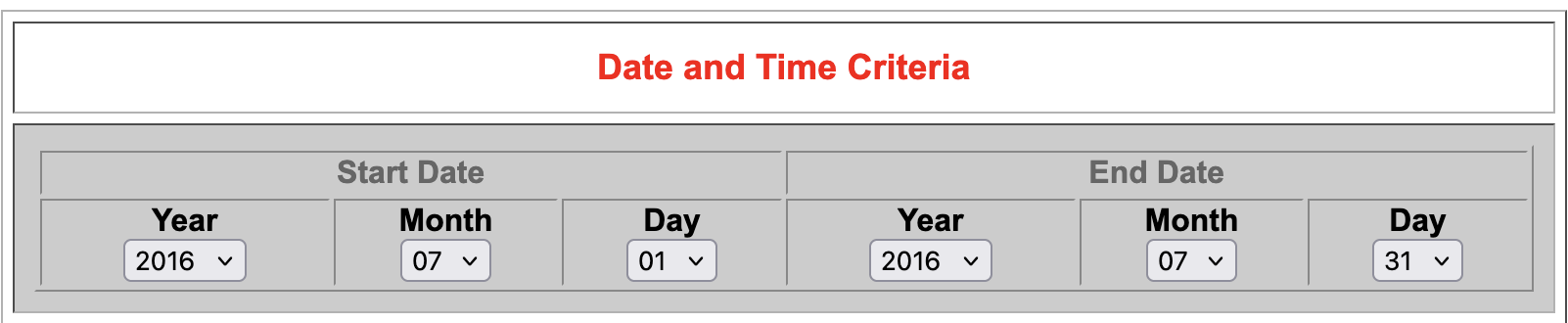
• Under Date and Time Criteria
  • Select Start Date
  • Year: 2016
  • Month: 07
  • Day: 01
  • Select End Date
  • Year: 2016
  • Month: 07
  • Day: 31

• Choose Program to Run
  • select Species Statistics and Spatial Plot(multi networks)
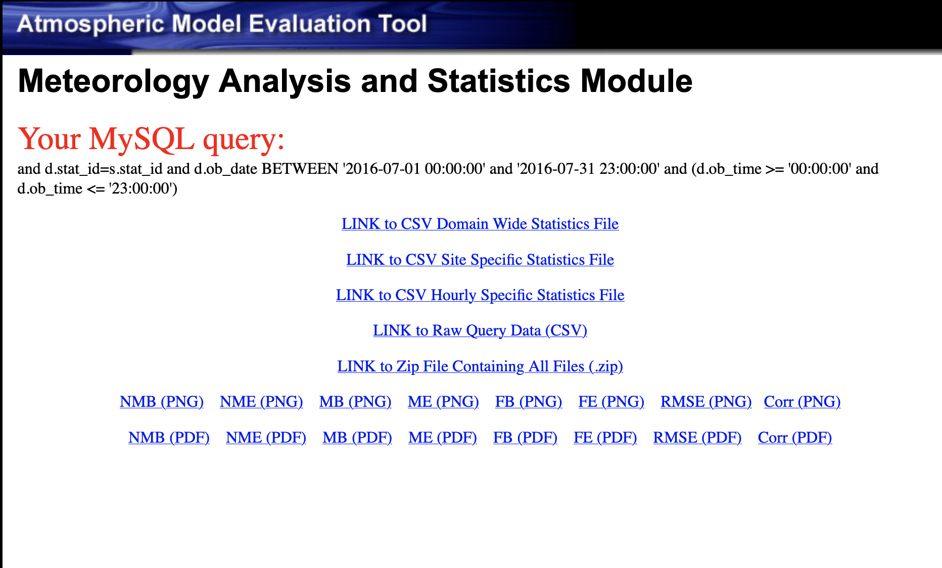
• Select Run Program

• Results of options selected in querygen_met.php

• 2m Temperature Normalized Mean Bias Plot

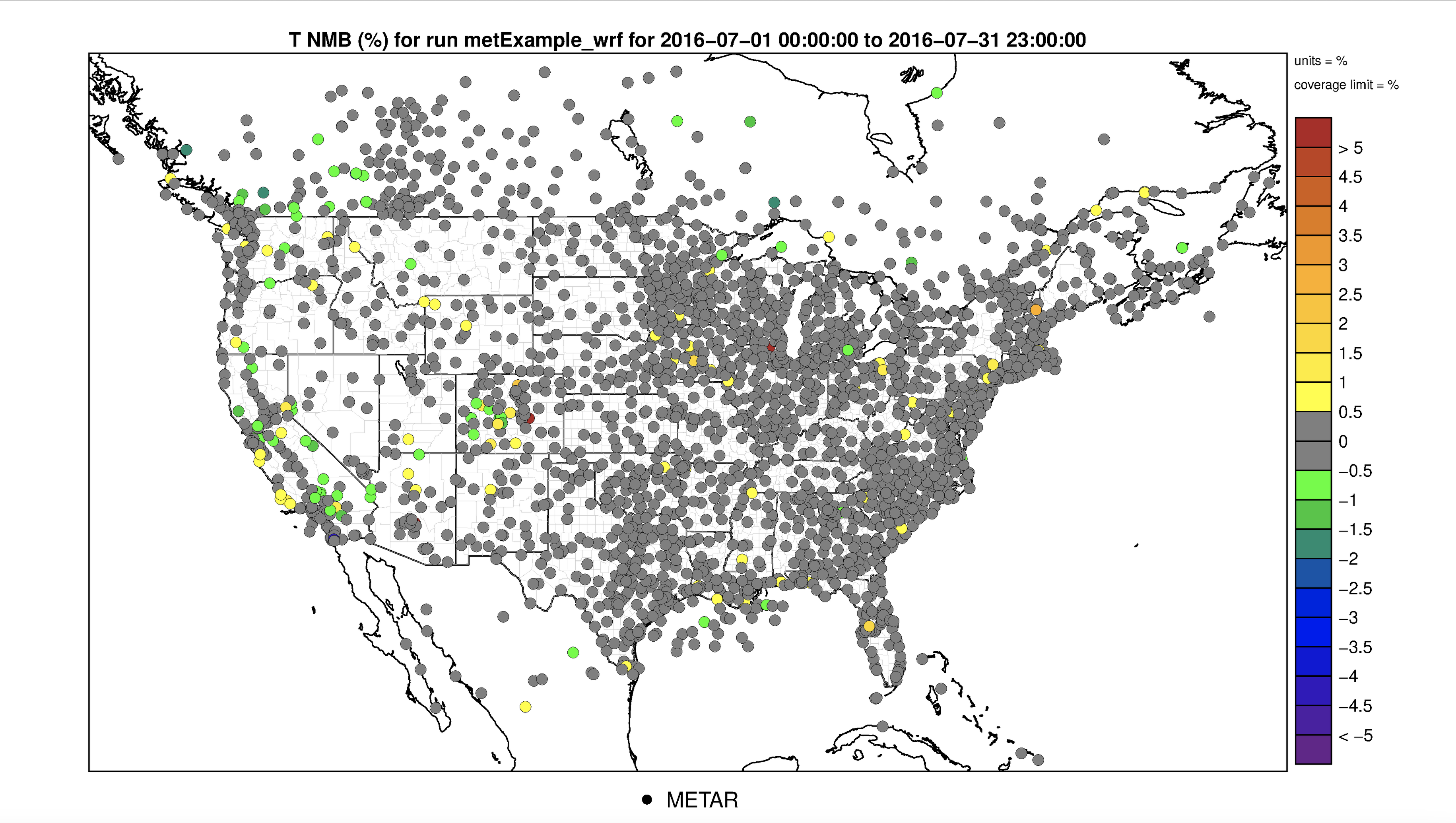
• 2m Temperature Normalized Mean Error Plot

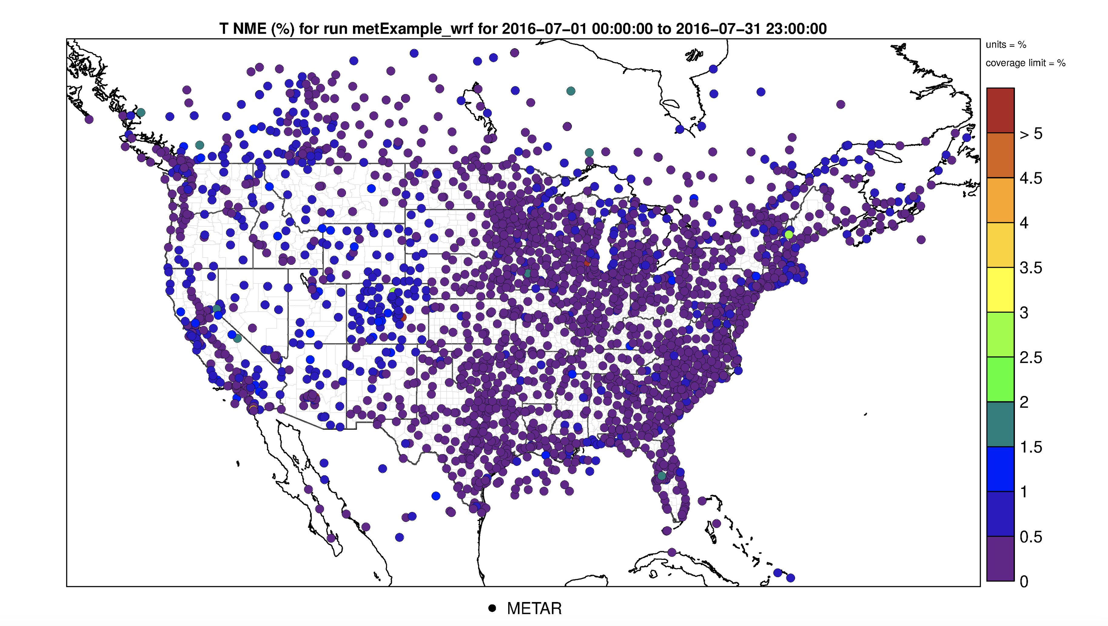
• 2m Temperature Mean Bias Plot

2m Temperature Mean Error Plot

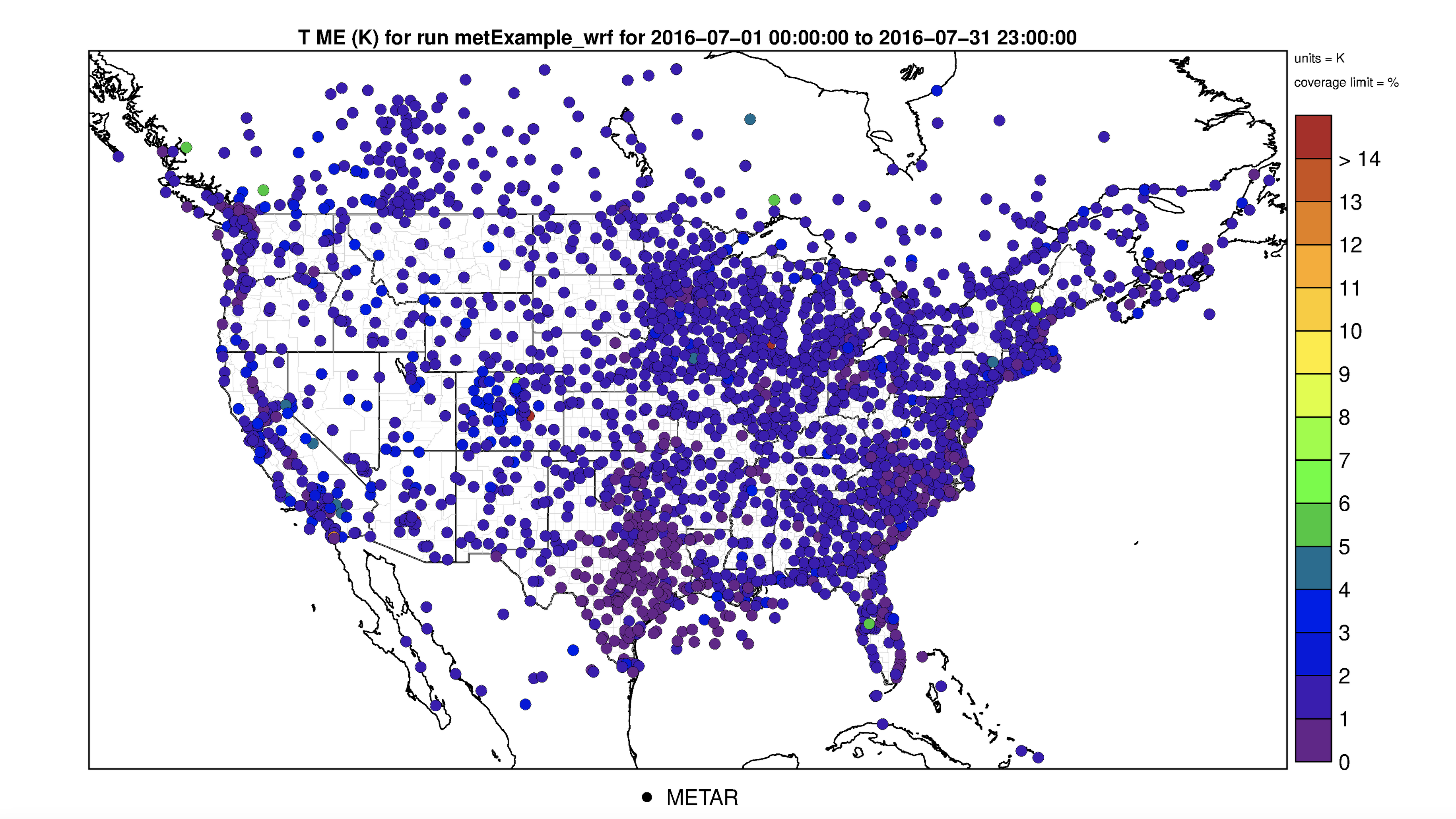
2m Temperature Root Mean Square Error Plot

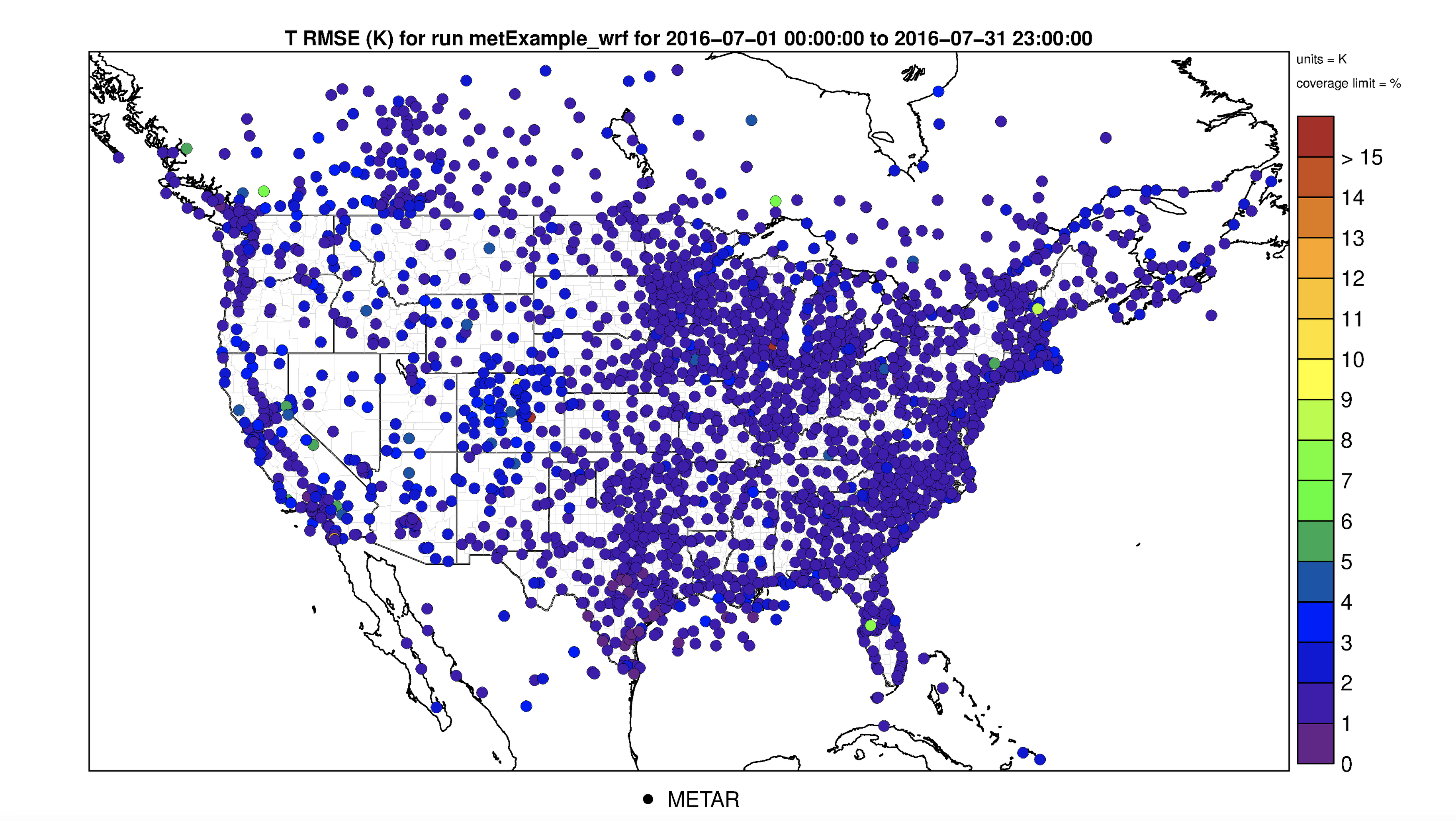
2m Temperature Correlation Plot

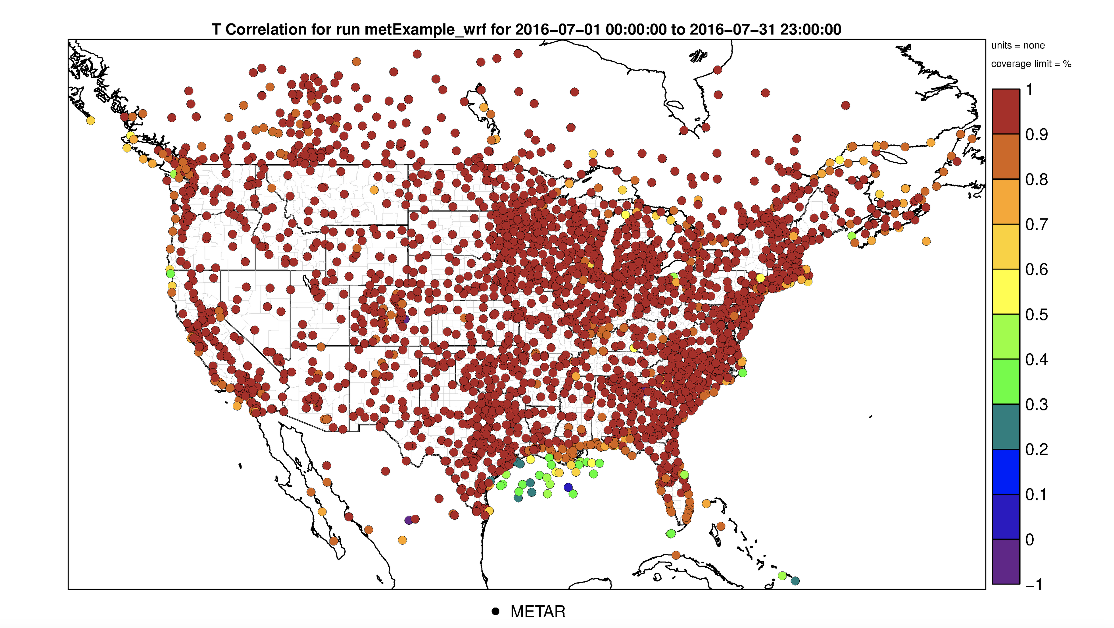
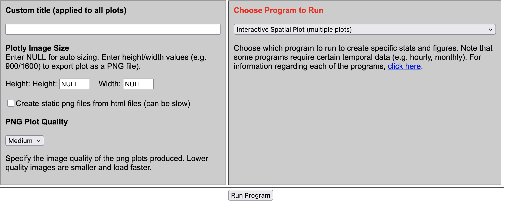
7.13.3. Create Interactive 2M Temperature Spatial Plots

• Under Met Variable to choose
  • Select T(2m)

• Under Choose Program to Run
  • Select Interactive Spatial Plot (multiple plots)

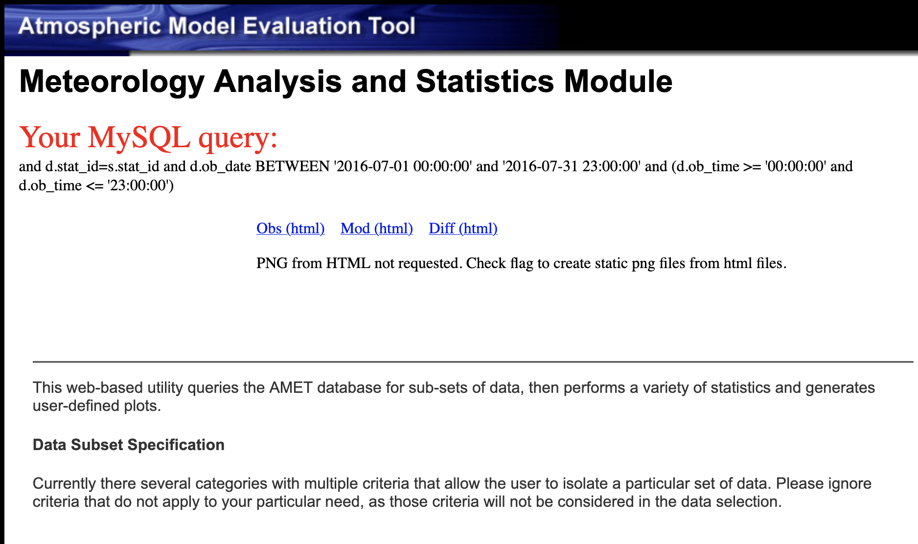
Results of options selected in querygen_met.php form

Spatial Plot of 2m Temperature Observations

Spatial Plot of 2m Temperature Model

Spatial Plot of 2m Temperature Difference between Model and Observations

7.13.4. Create Interactive 2M Temperature Spatial Plots using metExample_mpas

• Choose database
  • select amet
• Choose project 1
  • MetExample_mpas

• Under Met Variable to choose
  • Select T(2m)

• Under Choose Program to Run
  • Select Interactive Spatial Plot (multiple plots)

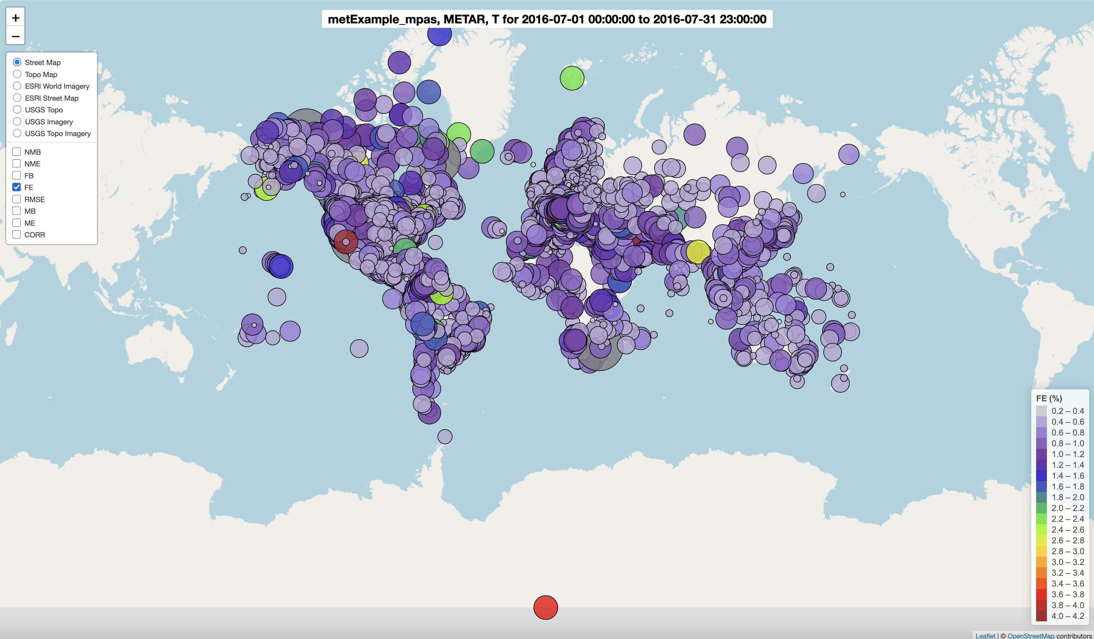
Interactive Spatial Plot of 2m Temperature Model/Observations NMB Statistic Selected

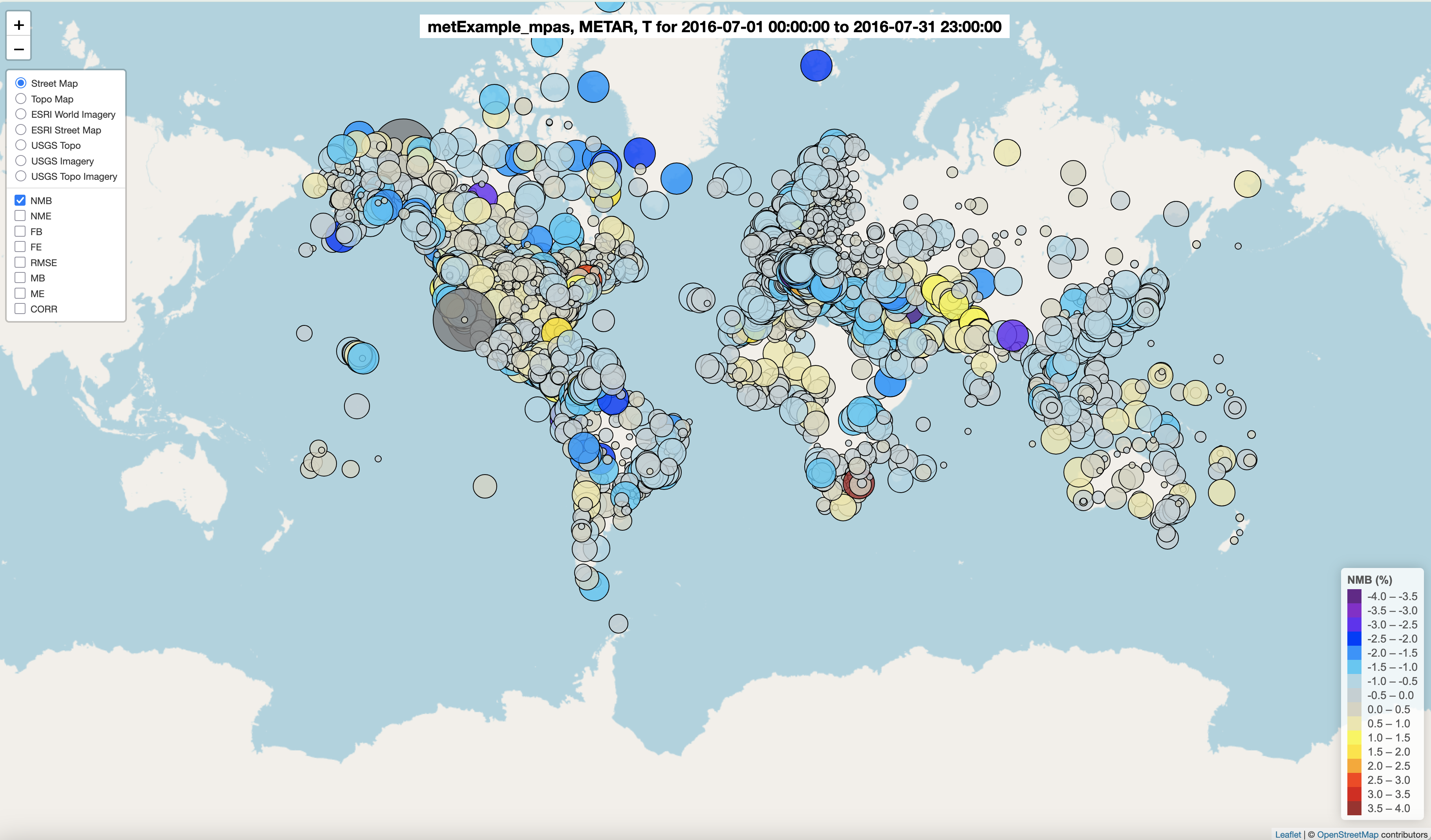
Spatial Plot of 2m Temperature Model/Observation NME Statistic Selected

Spatial Plot of 2m Temperature Model/Observations FB Statistic Selected

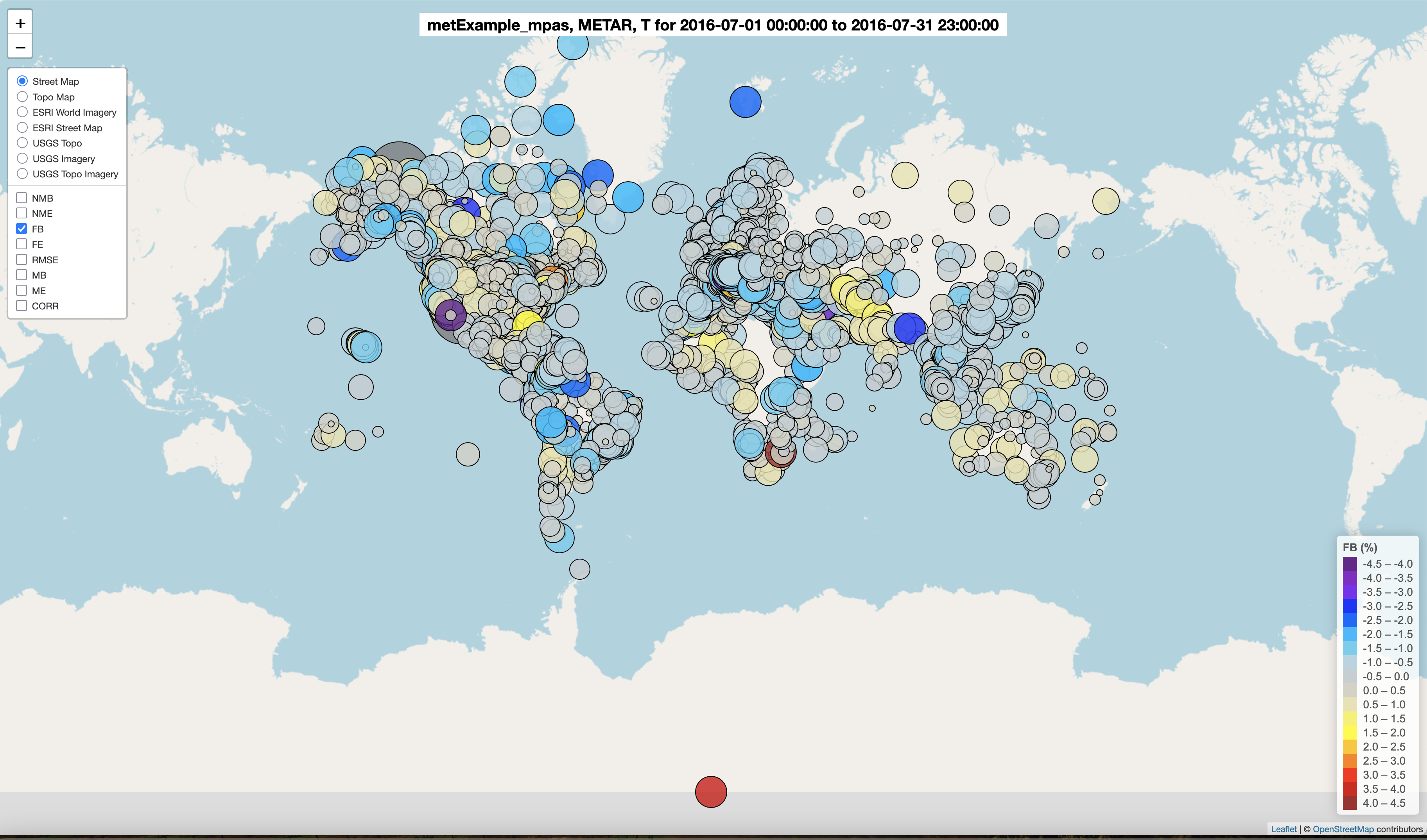
Spatial Plot of 2m Temperature Model/Observations FE Statistic Selected

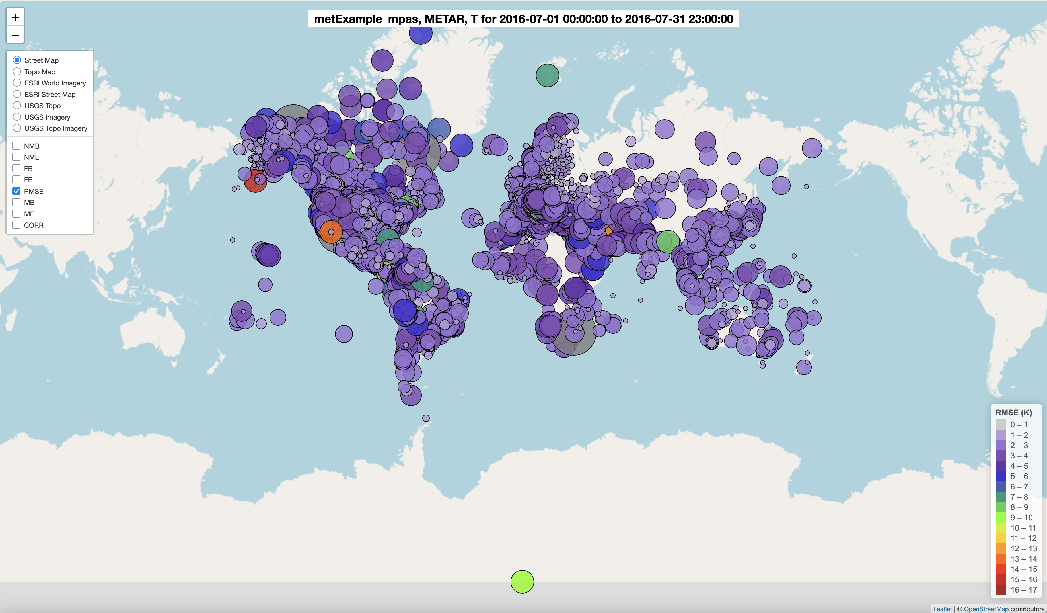
Spatial Plot of 2m Temperature Model/Observations RMSE Statistic Selected

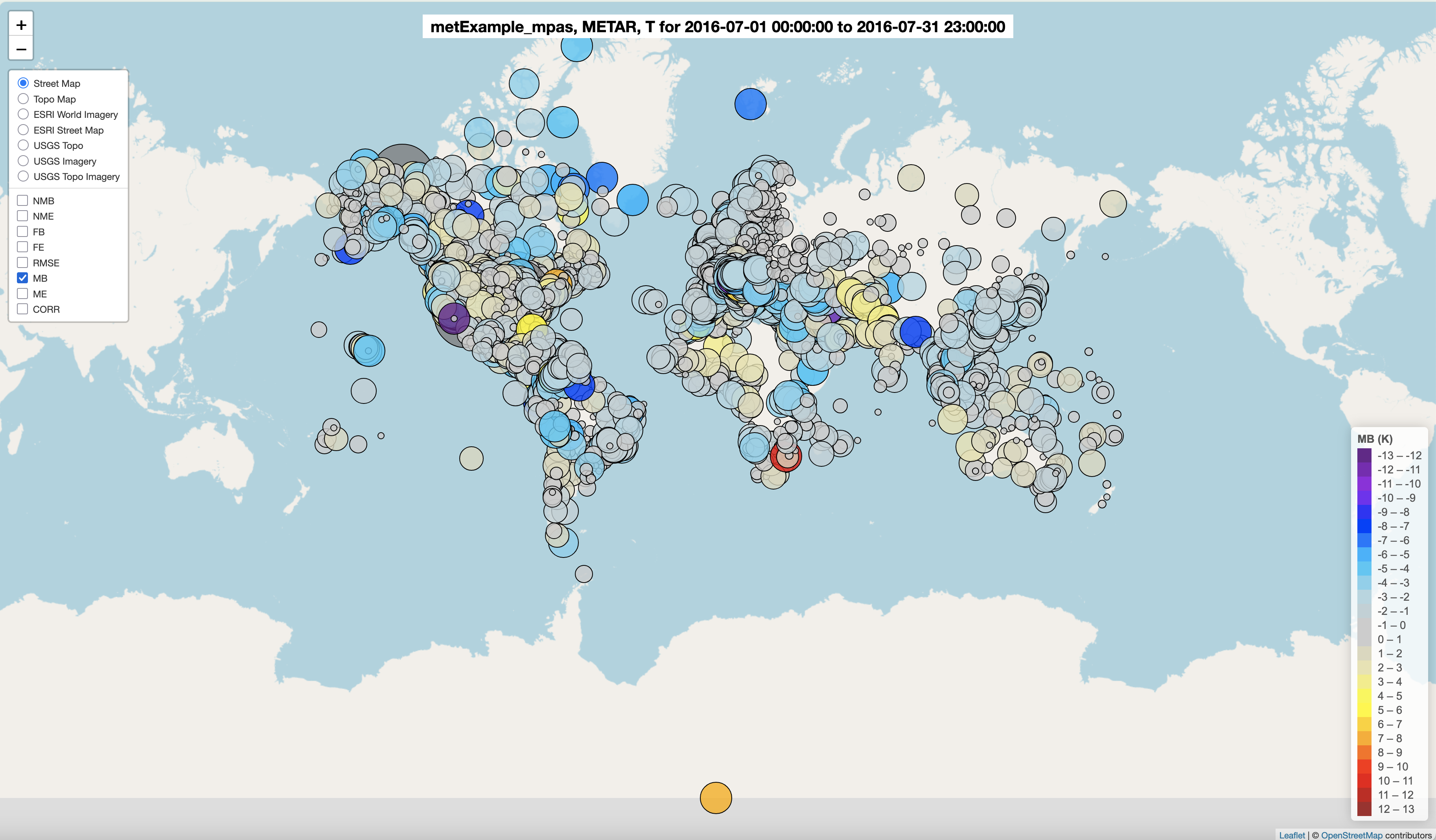
Spatial Plot of 2m Temperature Model/Observations MB Statistic Selected

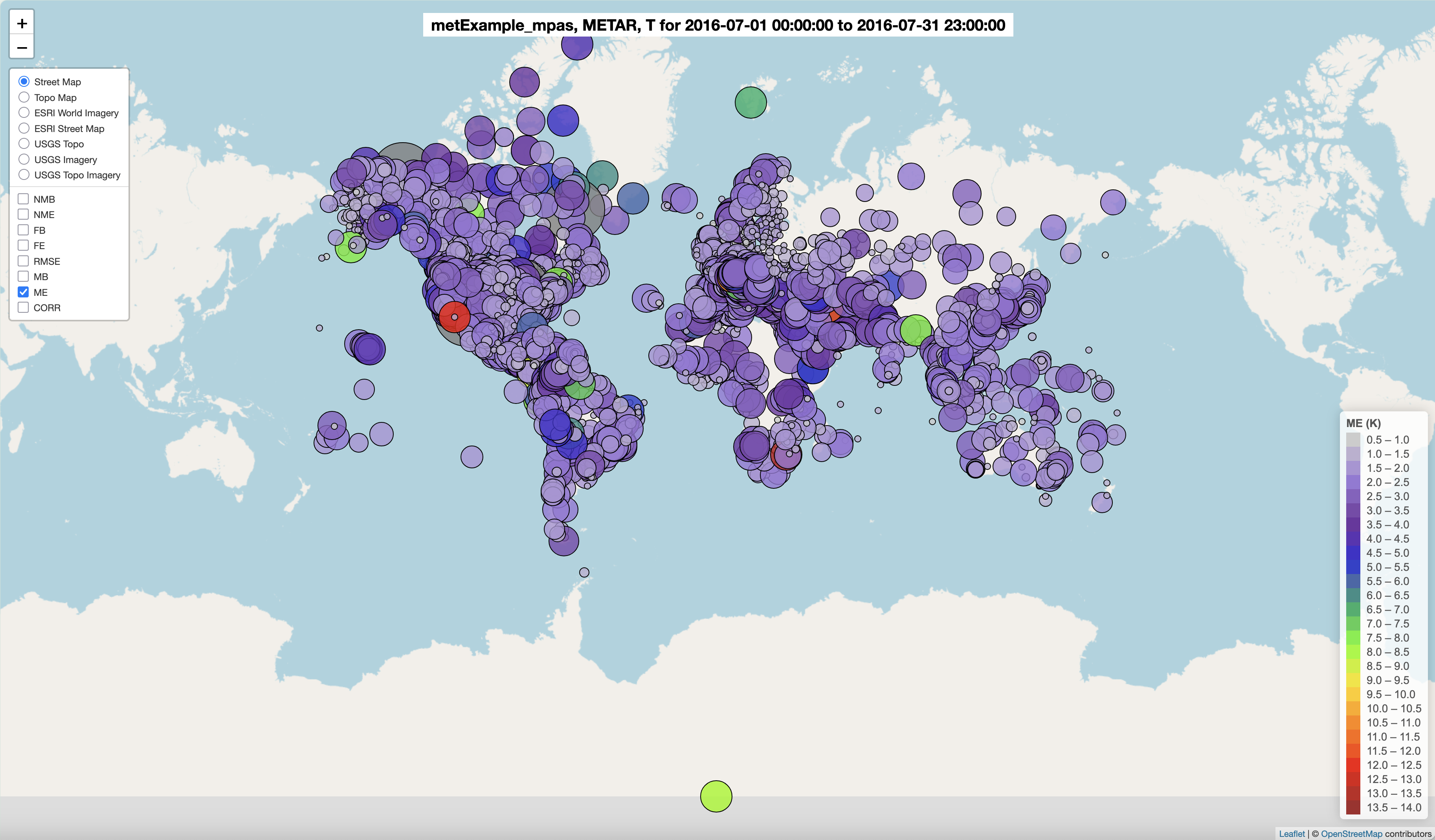
Spatial Plot of 2m Temperature Model/Observations ME Statistic Selected

Spatial Plot of 2m Temperature Model/Observations Corr Statistic Selected

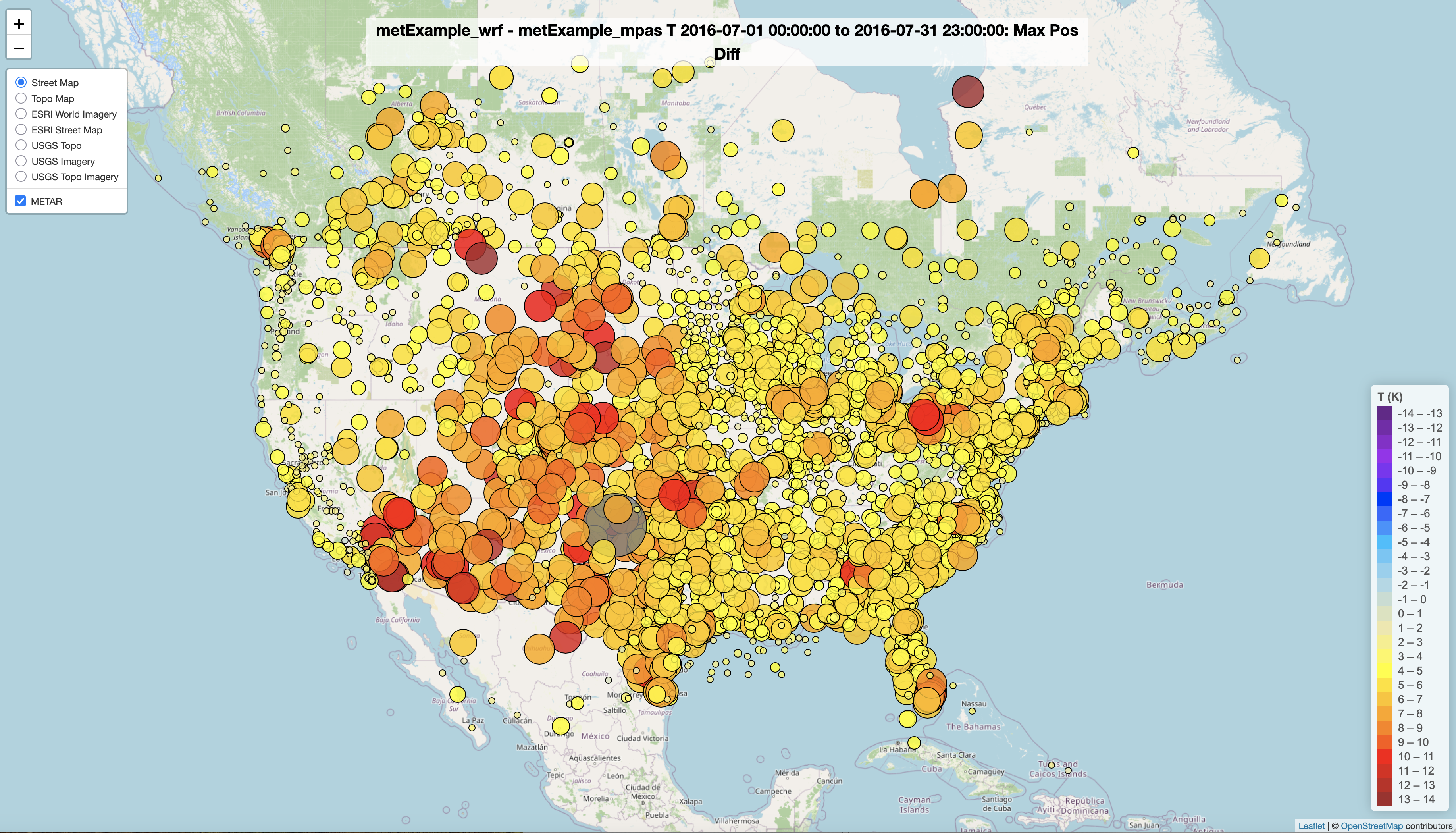
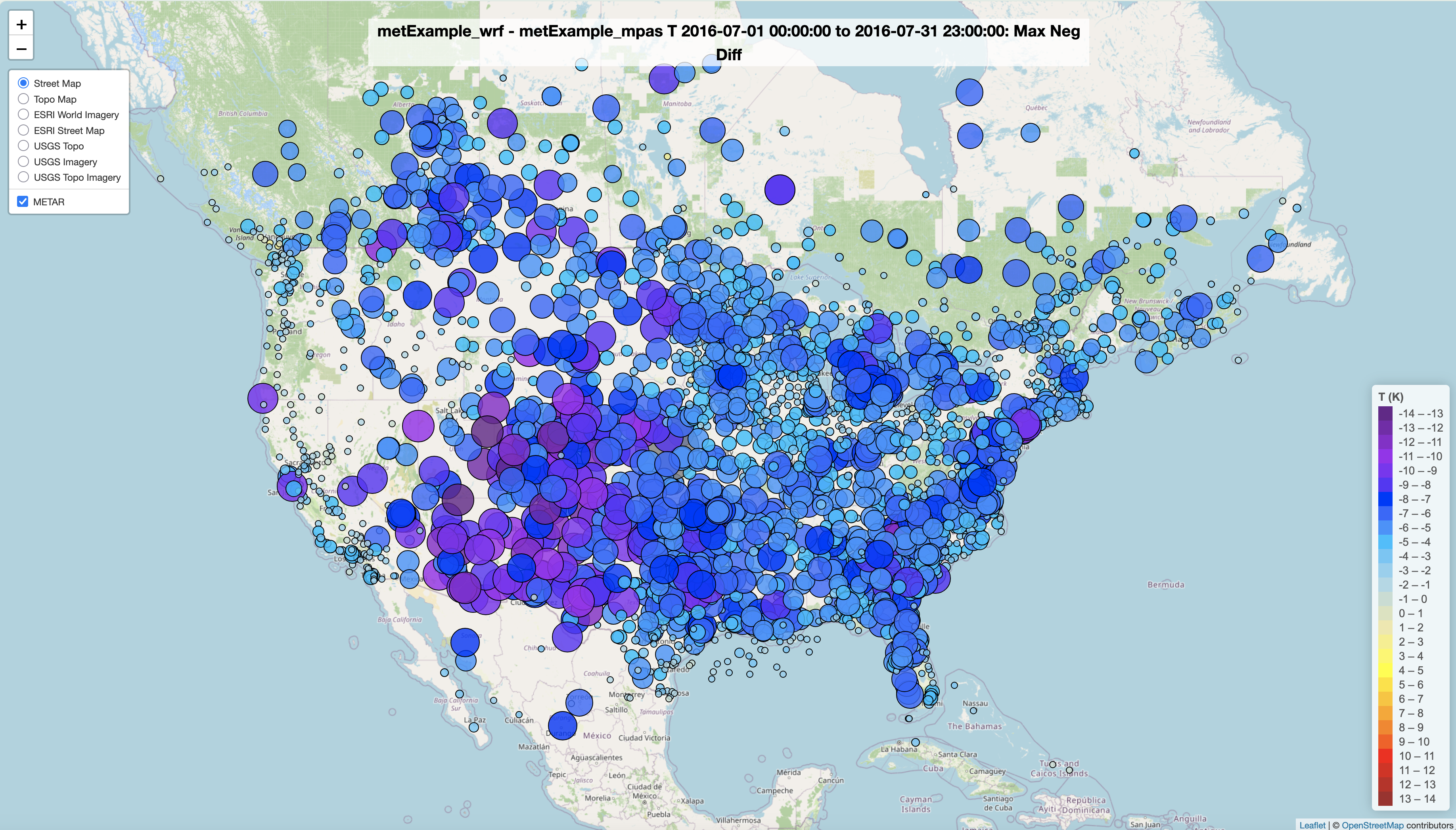
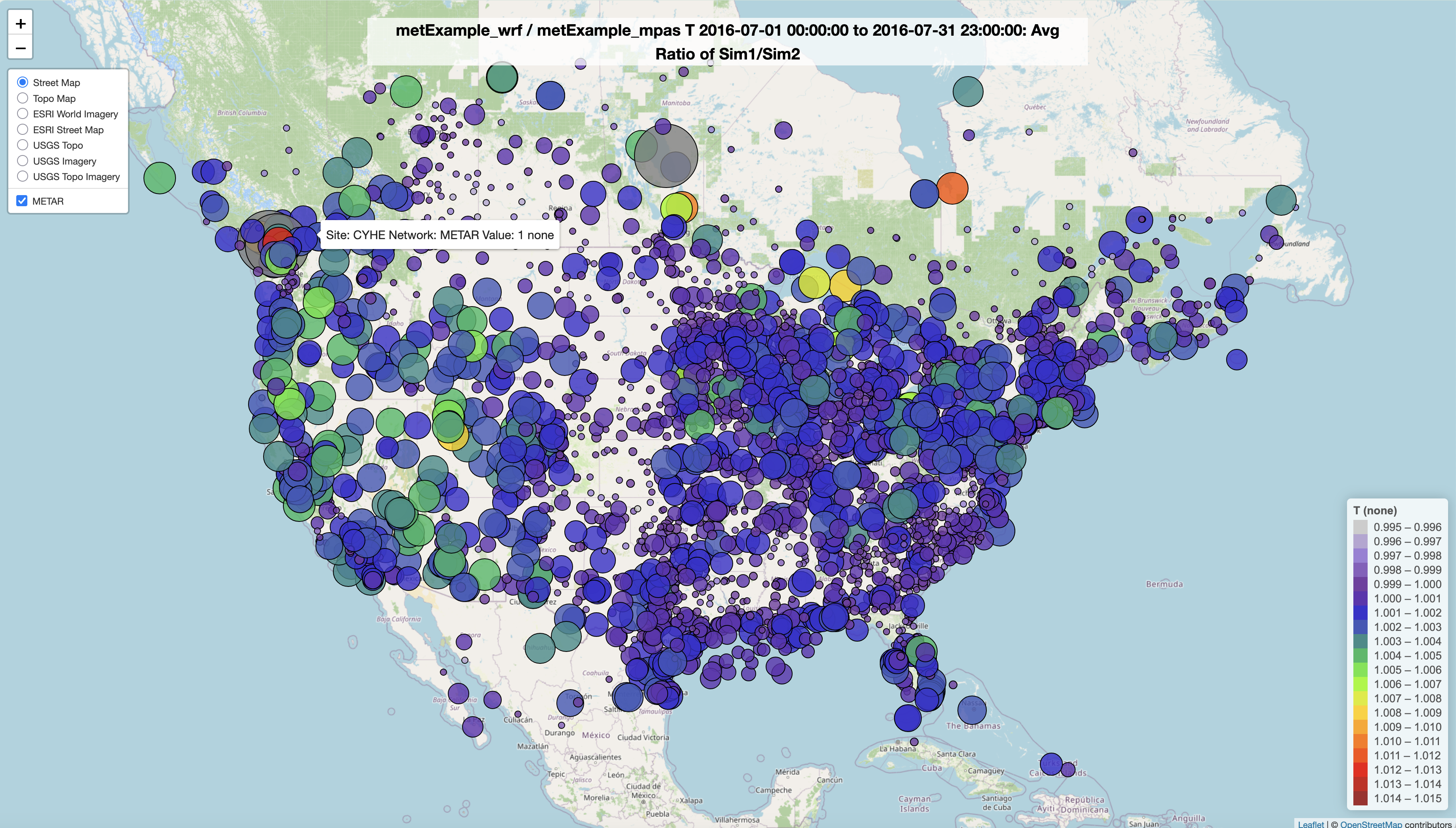
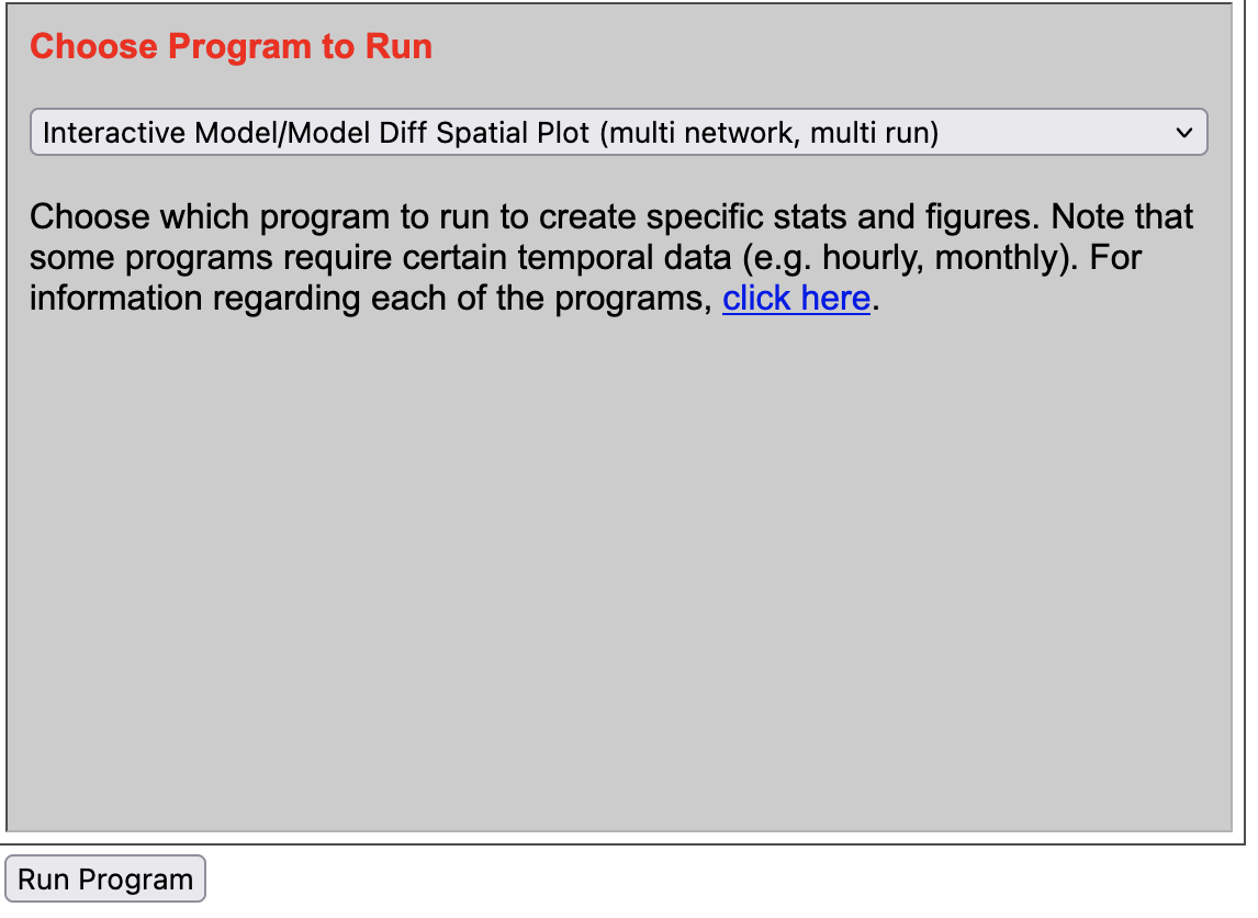
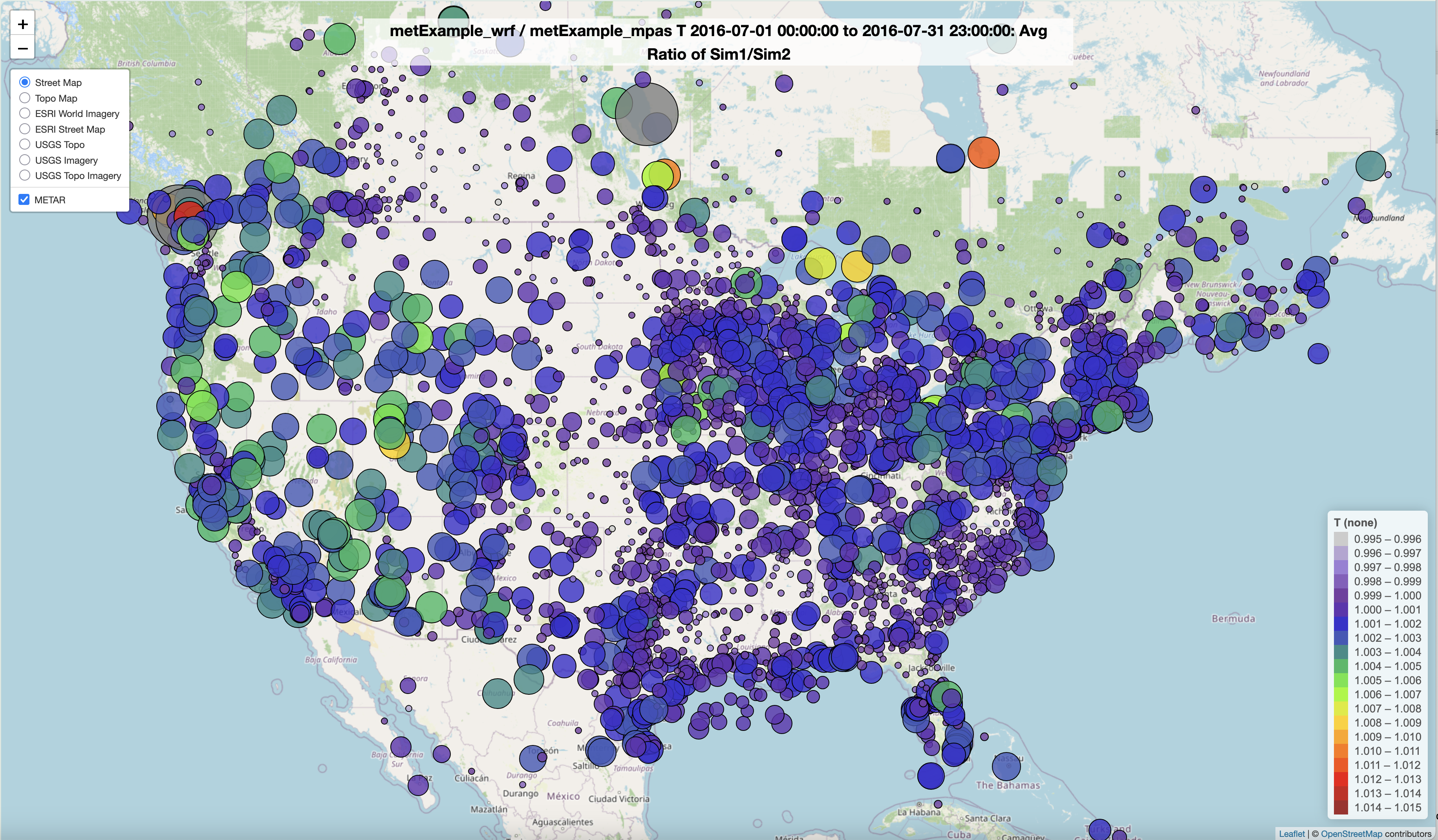
7.13.5. Create Interactive 2M Temperature Model to Model Difference Spatial Plots

• Under Met Variable to choose
  • Select T(2m)

• Under Choose Program to Run
  • Select Interactive Model to ModelSpatial Difference Plots (multi-networks, multi-run)

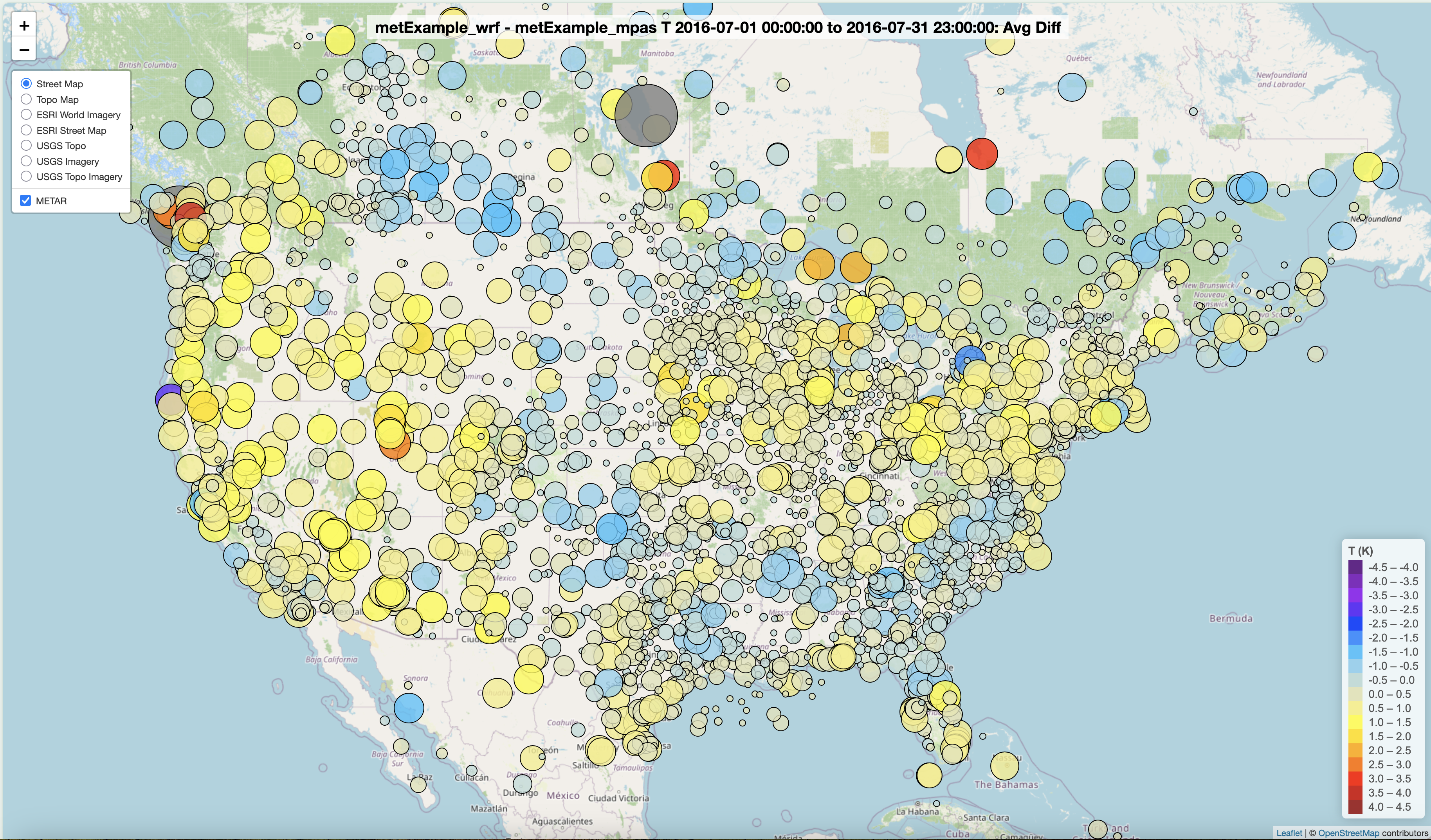
Results of options selected in querygen_met.php form

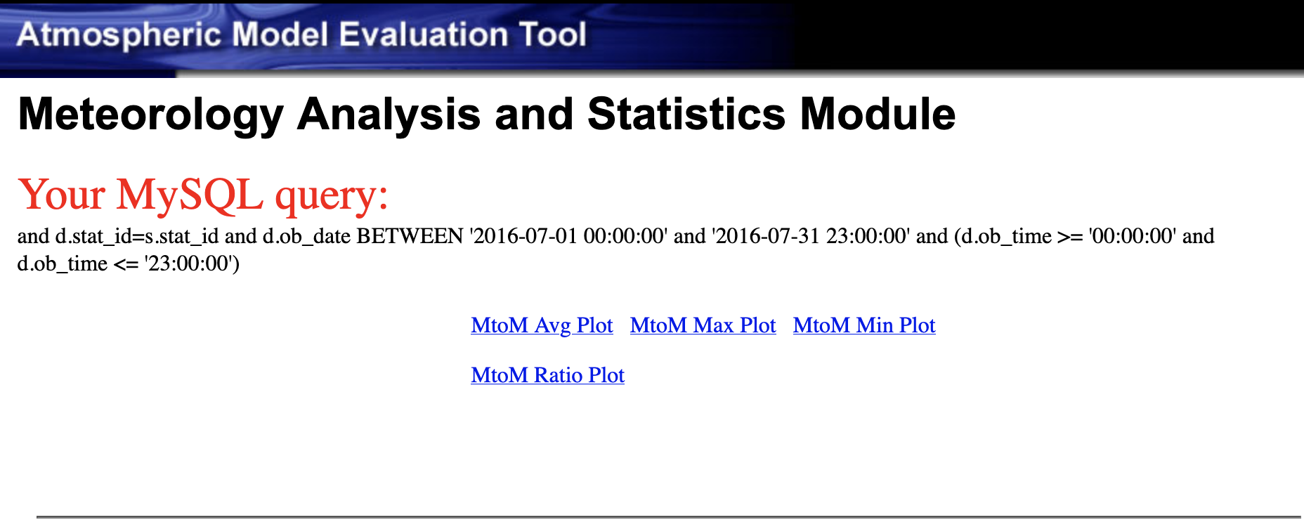
Spatial Plot of 2m Temperature Model to Model Average Difference Interactive Plot

Spatial Plot of 2m Temperature Model to Model Maximum Difference Interactive Plot

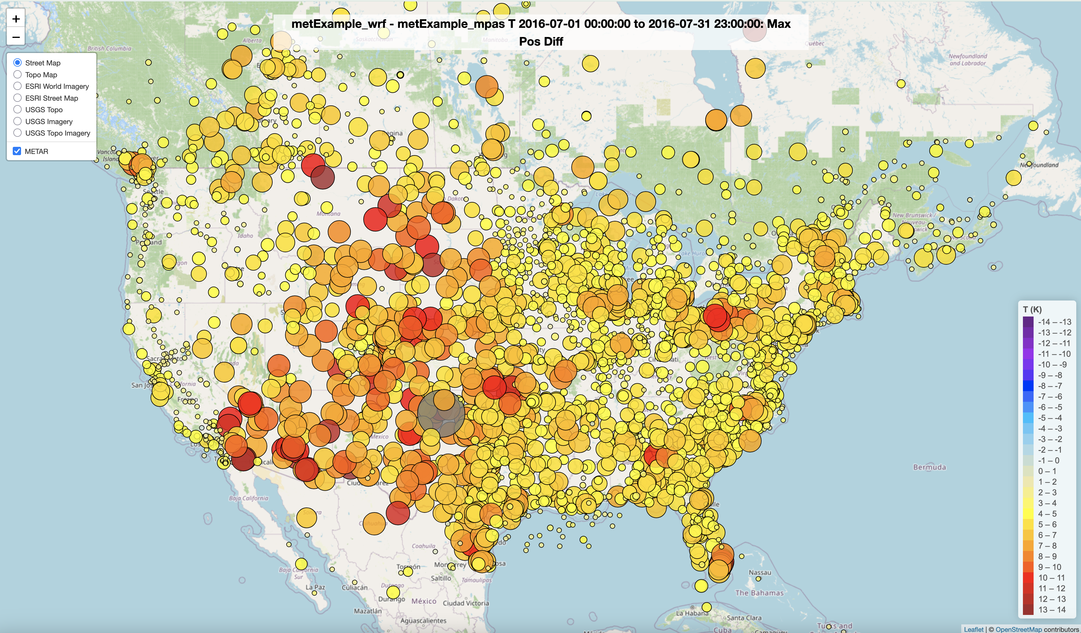
Spatial Plot of 2m Temperature Model to Model Minimum Difference Interactive Plot

Spatial Plot of 2m Temperature Model to Model Difference Ratio Interactive Plot

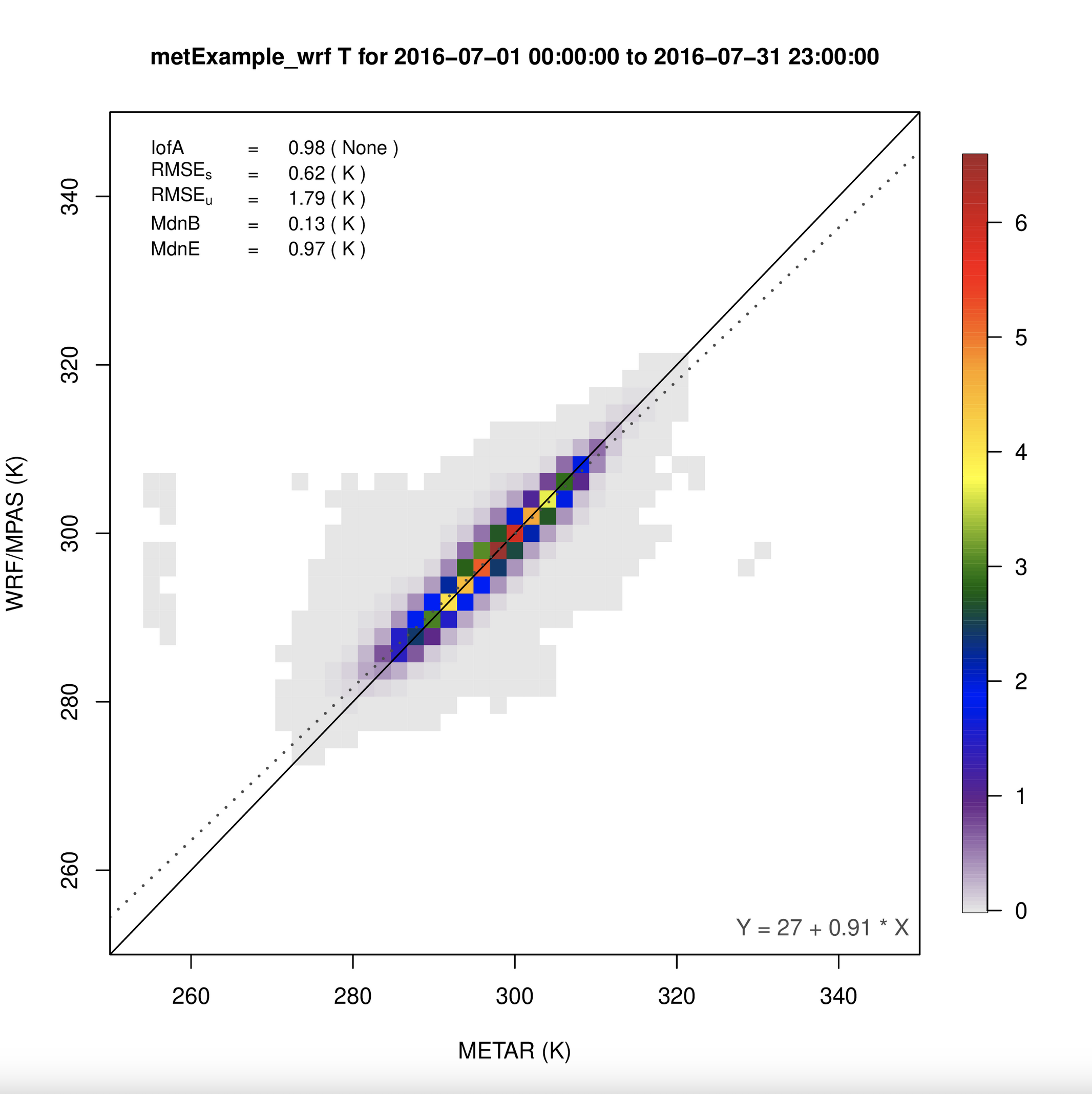
7.13.6. Create 2m Temperature Density Scatterplot

• Under Met Variable to choose
  • Select T(2m)

• Under Data Format and Plot Specifications, Under AMET Plots Axis Options
  • Select x-axis min
  • 250
  • Select x-axis max
  • 350
  • Select y-axis min
  • 250
  • Select y-axis max
  • 350

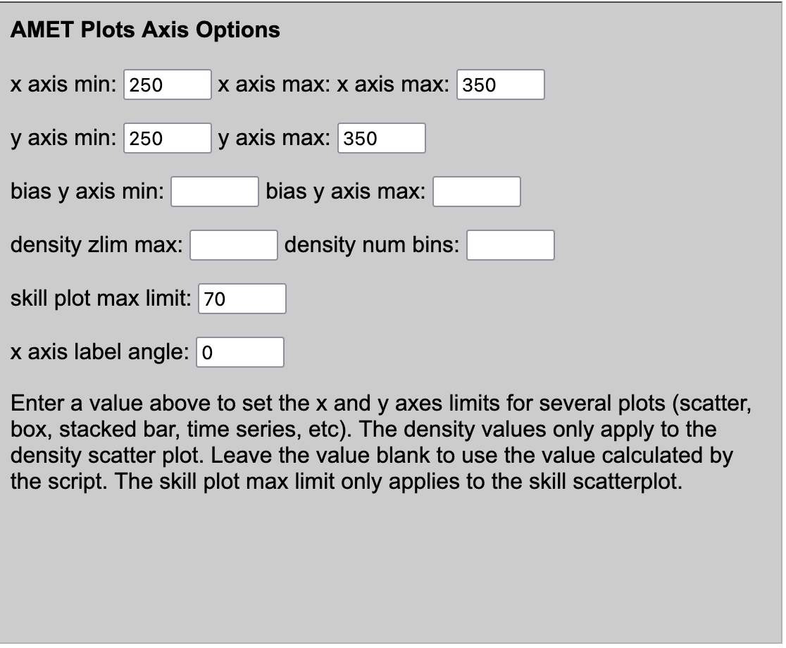
• Under Choose Program to Run
  • Select Density Scatterplot (single run, single network)

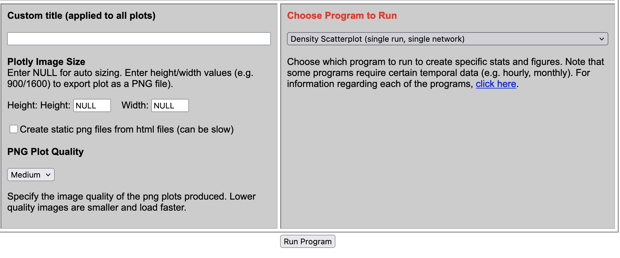
Results of options selected in querygen_met.php form

Scatterplot of 2m Temperature metExample_wrf vs METAR

Scatterplot of 2m Temperature metExample_mpas vs METAR

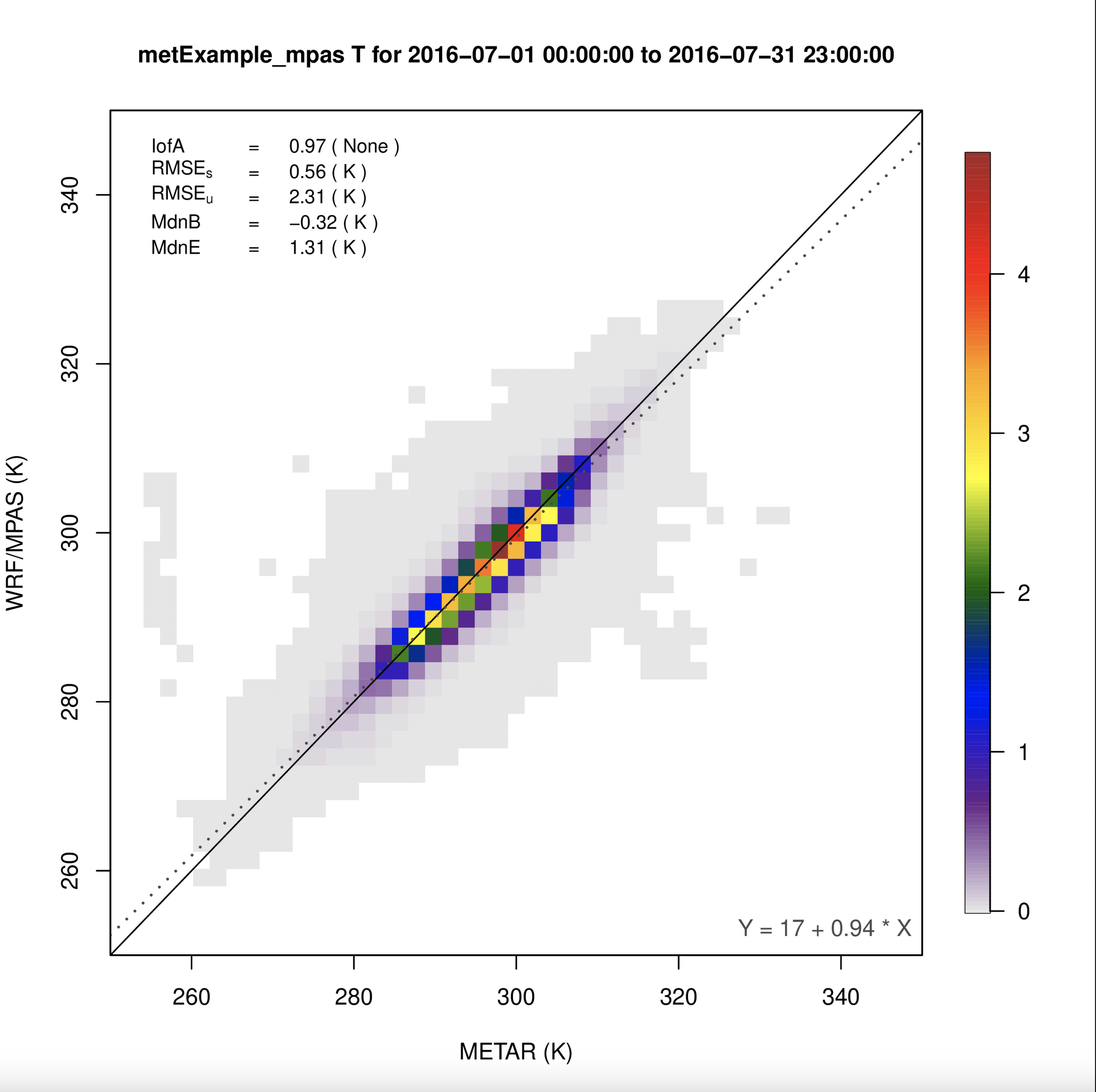
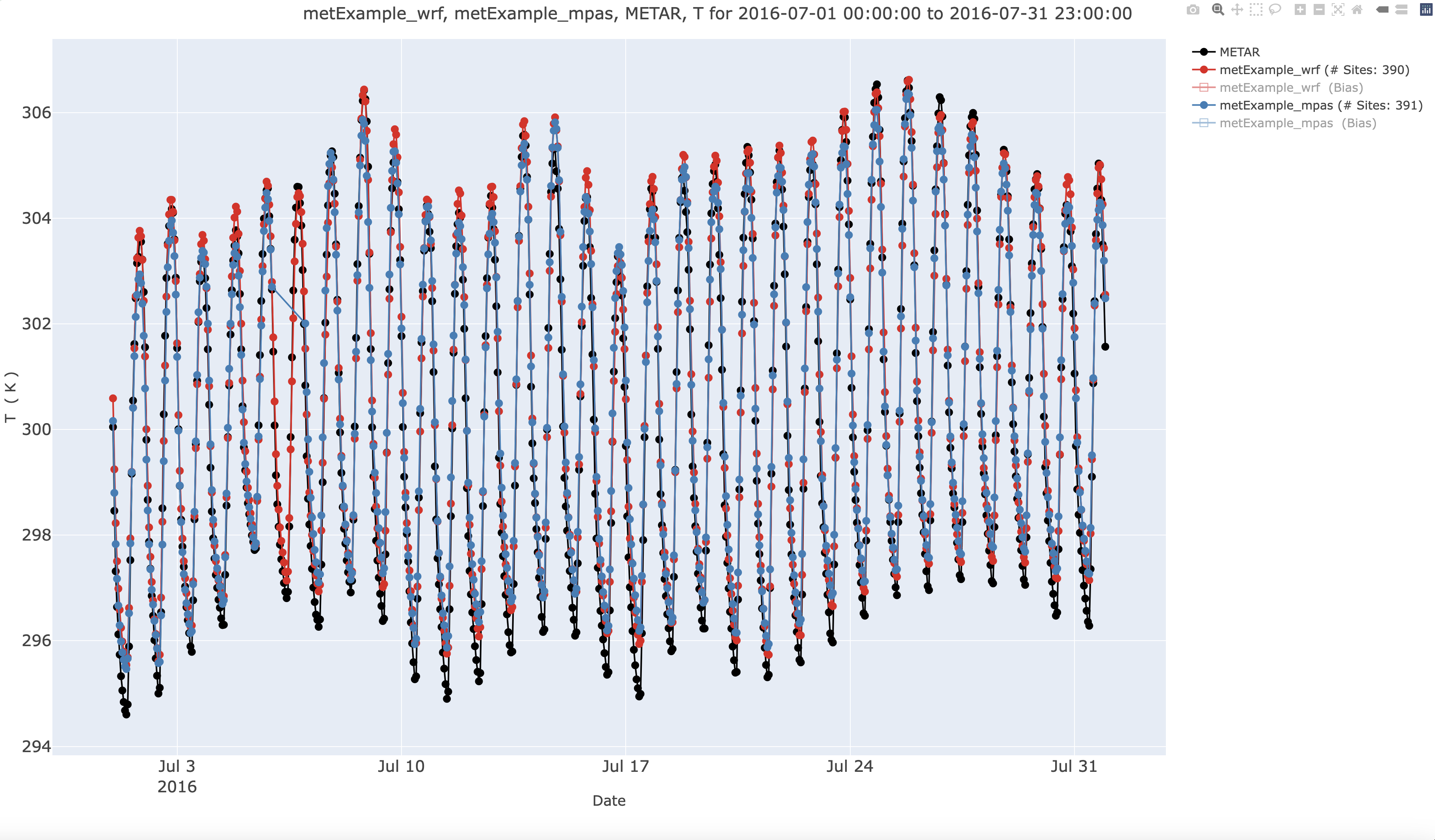
Notice that the range of temperatures for mpas is much larger than for wrf. 260 K is 8 deg. Farenheit, do MPAS/METAR model-obs values exist in July? Perhaps in the artic, or in the southern hemisphere (where it is winter). Restrict the area used, to be all of the Regional Planning Office Regions (all of the US states) and replot the scatterplots for both wrf and mpas. The METAR stations are world-wide, and MPAS model also covers the globe. Recommend that comparisons of T2 (surface temperature) from the WRF and MPAS models be done over similar spatial areas. First select a state, or region of interest, in this case the selection is for all of the Regional Planning Office regions.

Scatterplot of 2m Temperature metExample_wrf vs METAR restricted to RPO Regions (United States)

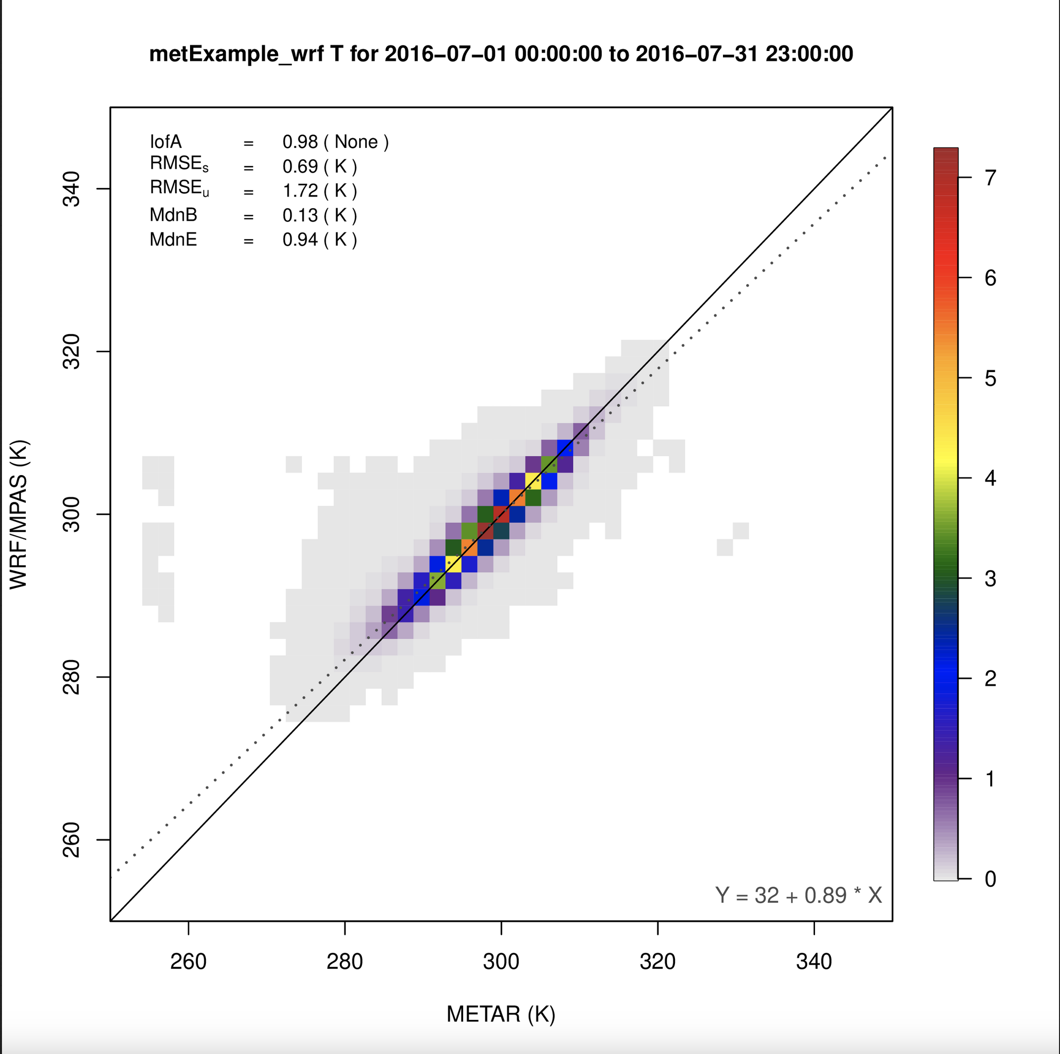
Scatterplot of 2m Temperature metExample_mpas vs METAR restricted to RPO Regions (United States)

7.13.7. Create Timeseries Plot (single network, multiple sites averaged) for 2m Temperature

• Under Met Variable to choose
  • Select T(2m)

• Under Date and Time Criteria
  • Select Start Date
  • Year: 2016
  • Month: 07
  • Day: 01
  • Select End Date
  • Year: 2016
  • Month: 07
  • Day: 31

• Under Choose Program to Run
  • Timeseries Plot (single network, multiple sites averaged)

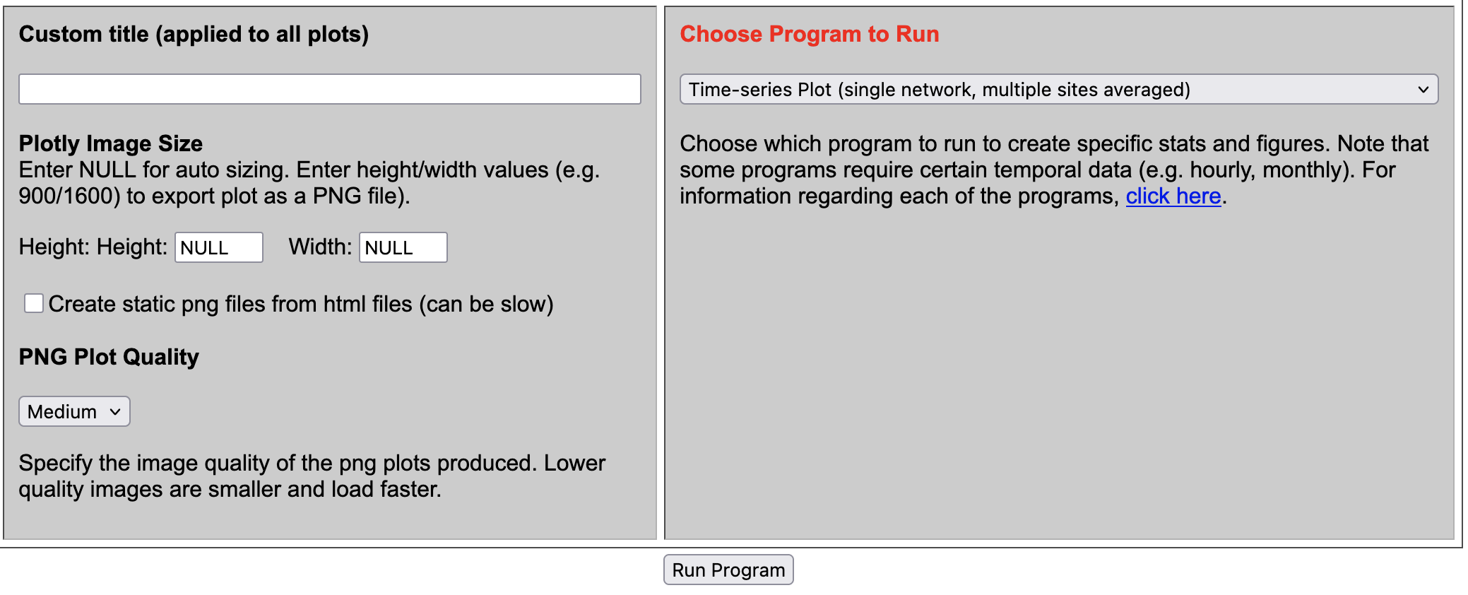
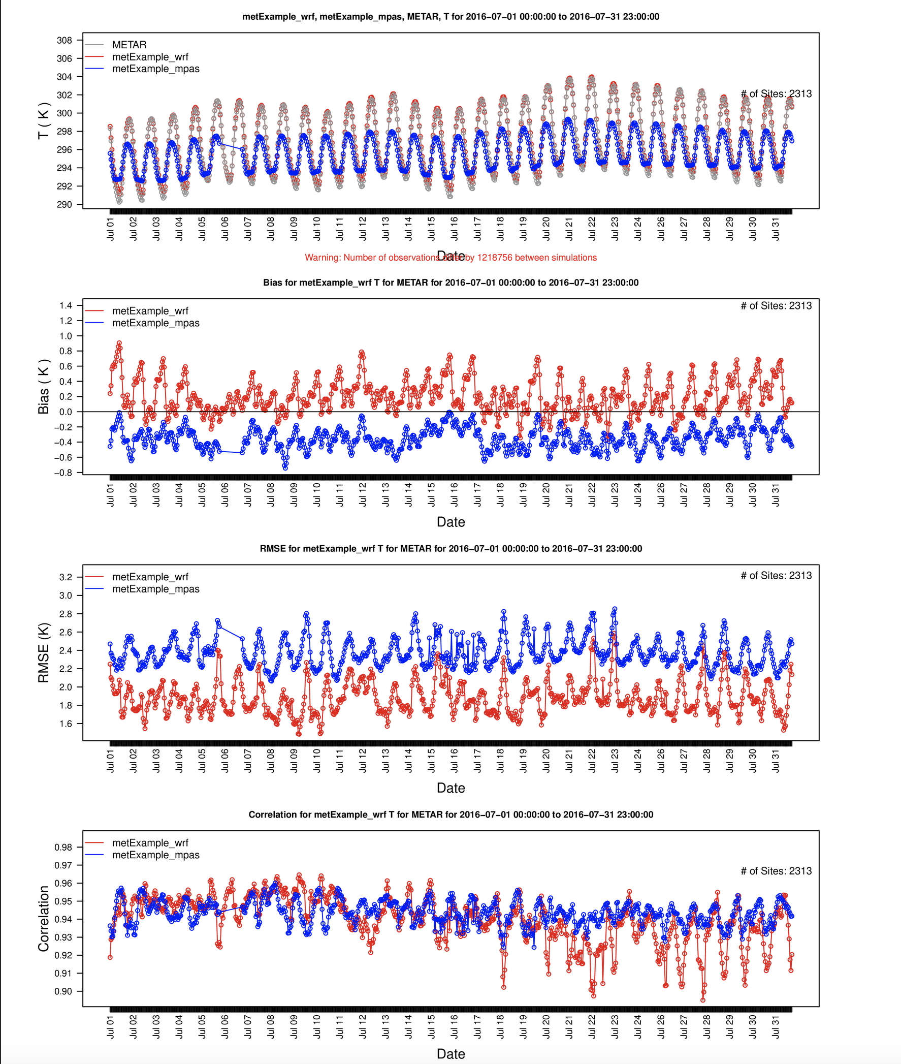
Results of options selected in querygen_met.php form

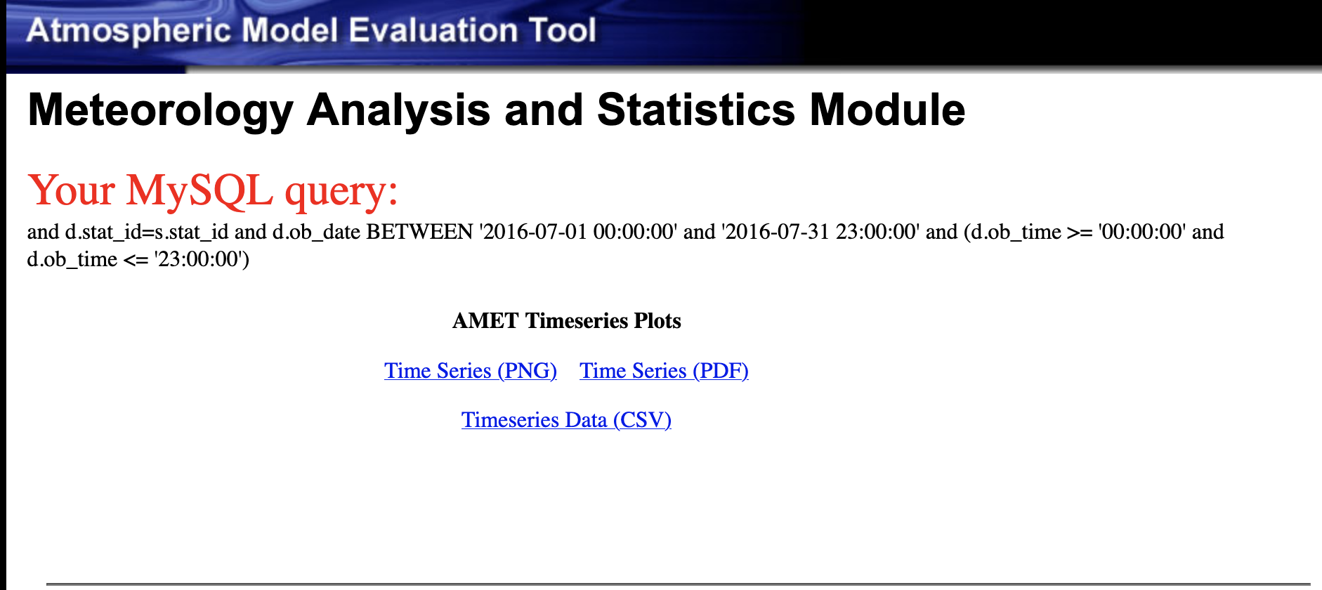
Timeseries Plot of 2m Temperature

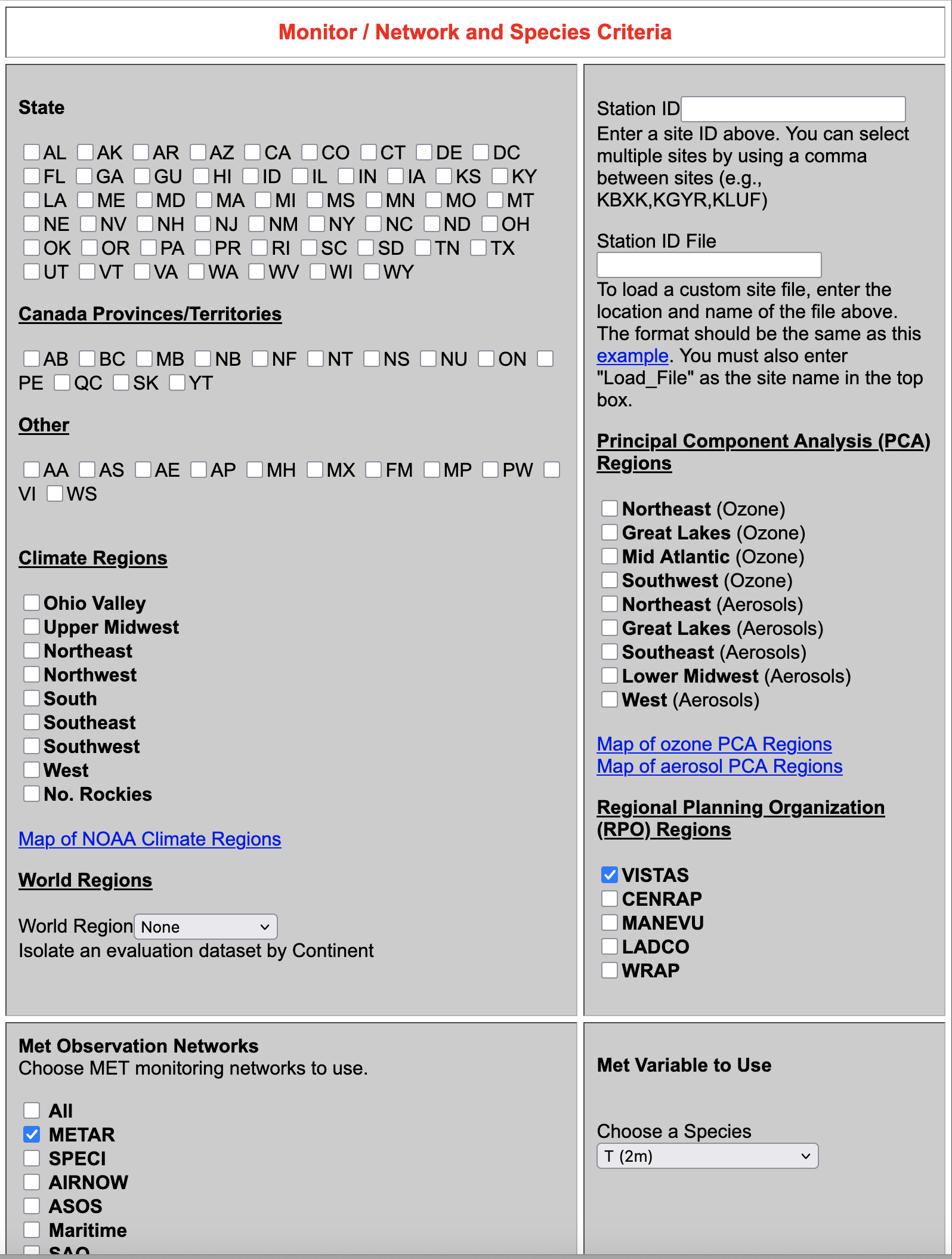
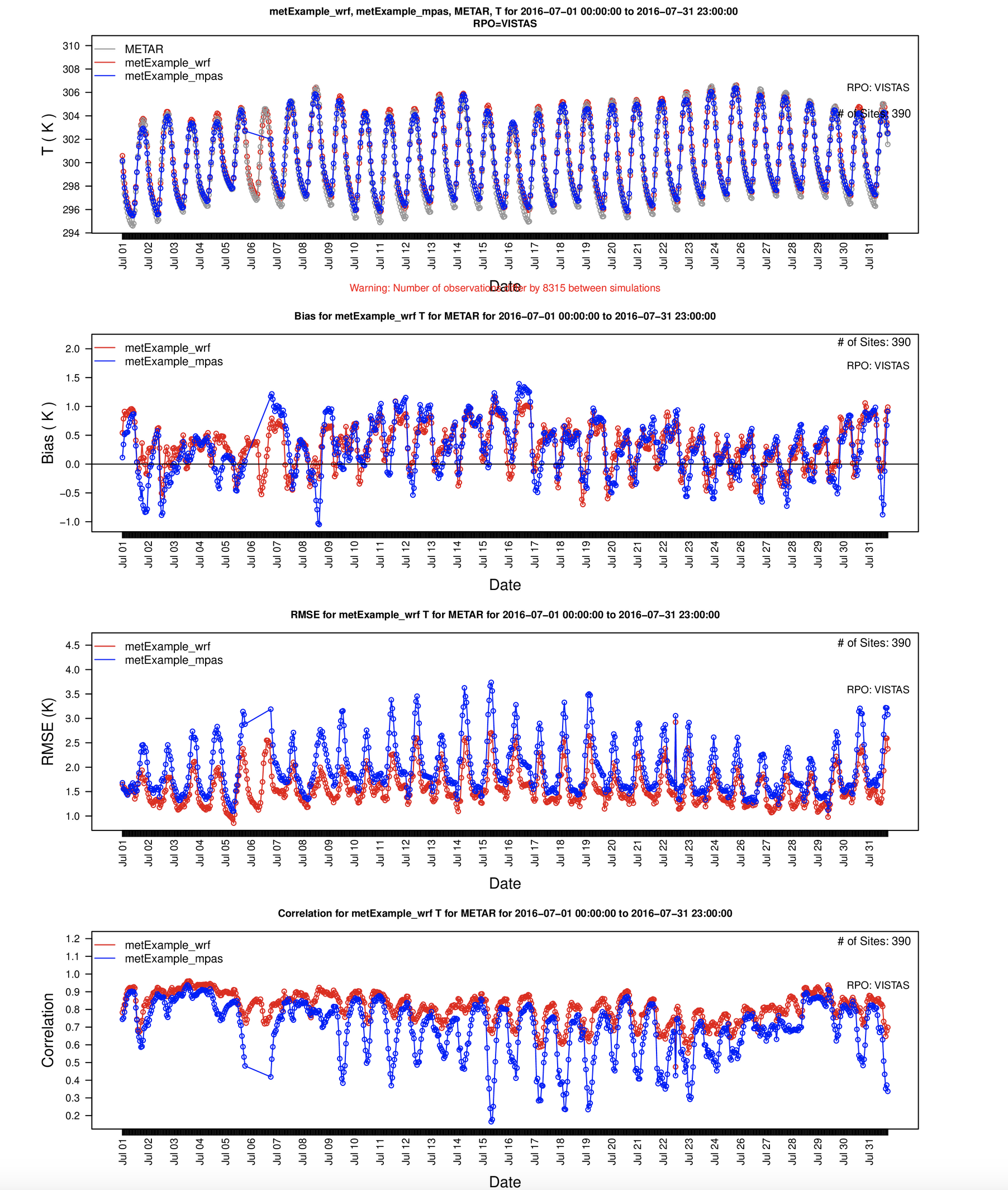
7.13.8. Create Timeseries Plot (single network, multiple sites averaged) for 2m Temperature for Select Region

• Under Met Variable to choose
  • Select T(2m)

• Monitor / Network and Species Criteria
  • Select VISTAS RPO

• Under Date and Time Criteria
  • Select Start Date
  • Year: 2016
  • Month: 07
  • Day: 01
  • Select End Date
  • Year: 2016
  • Month: 07
  • Day: 31

• Under Choose Program to Run
  • Timeseries Plot (single network, multiple sites averaged)

Results of options selected in querygen_met.php form

Timeseries Plot of 2m Temperature for VISTAS RPO Region

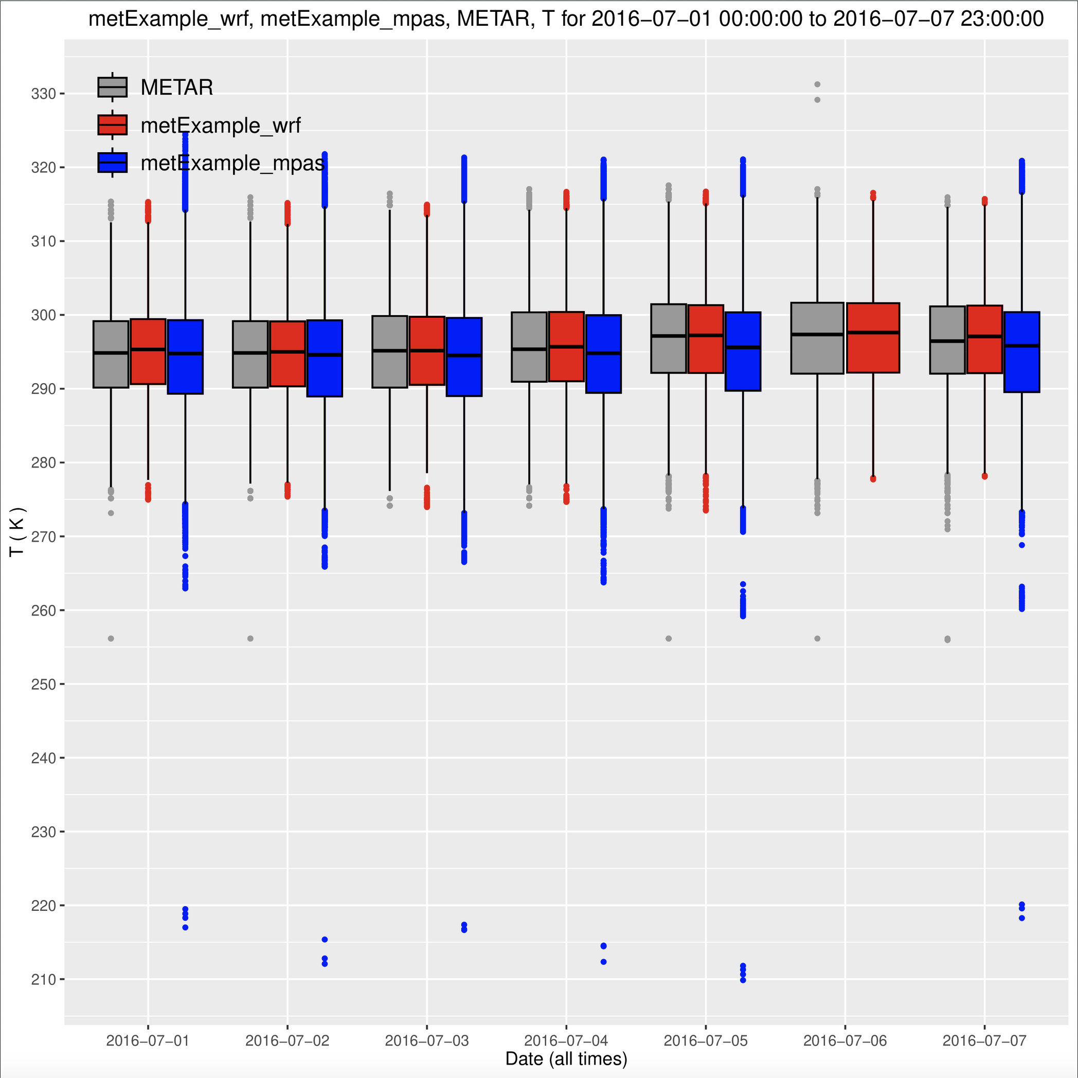
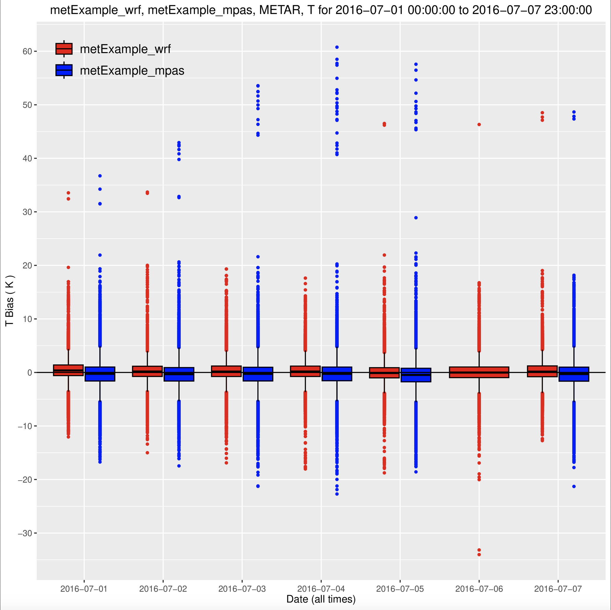
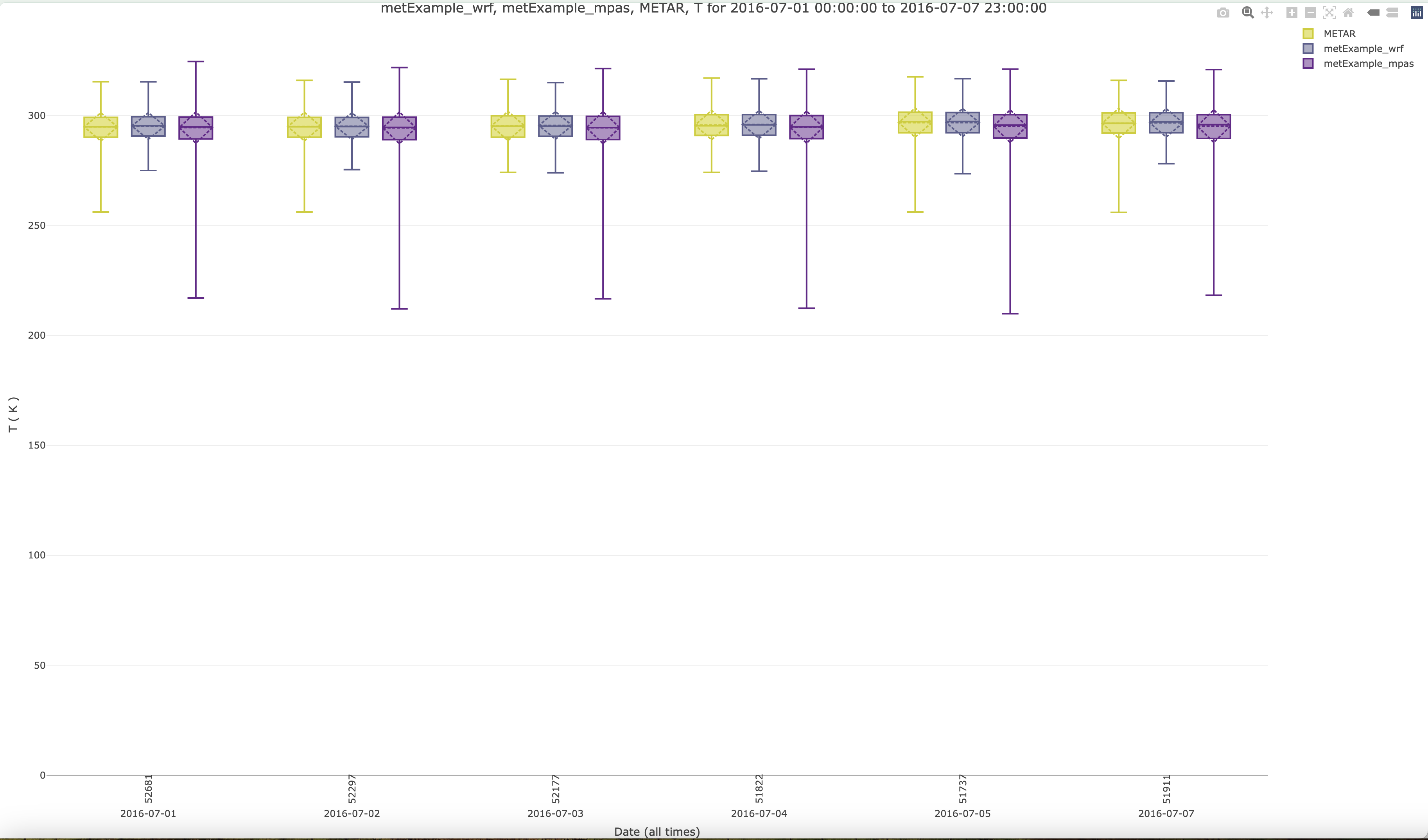
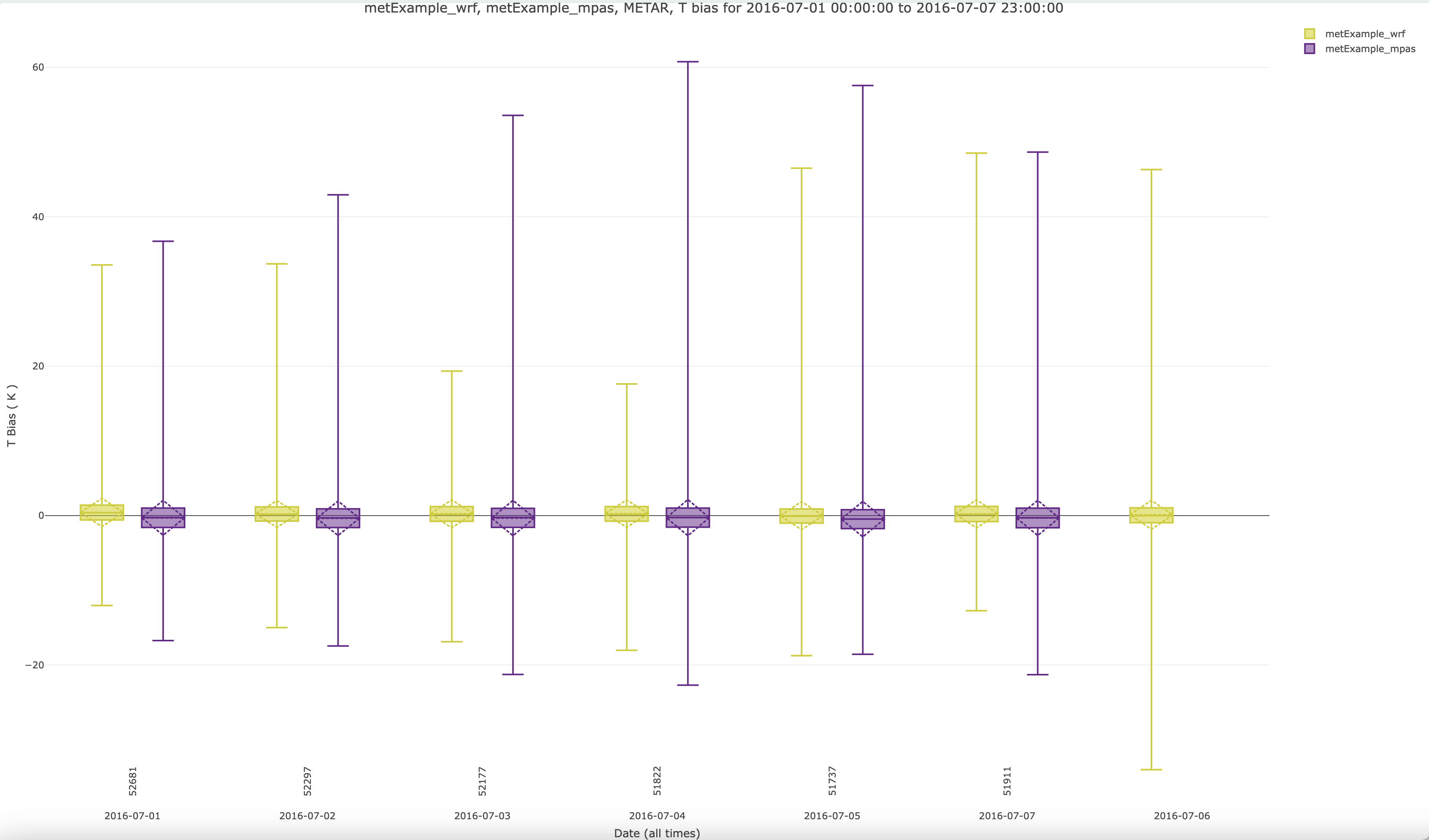
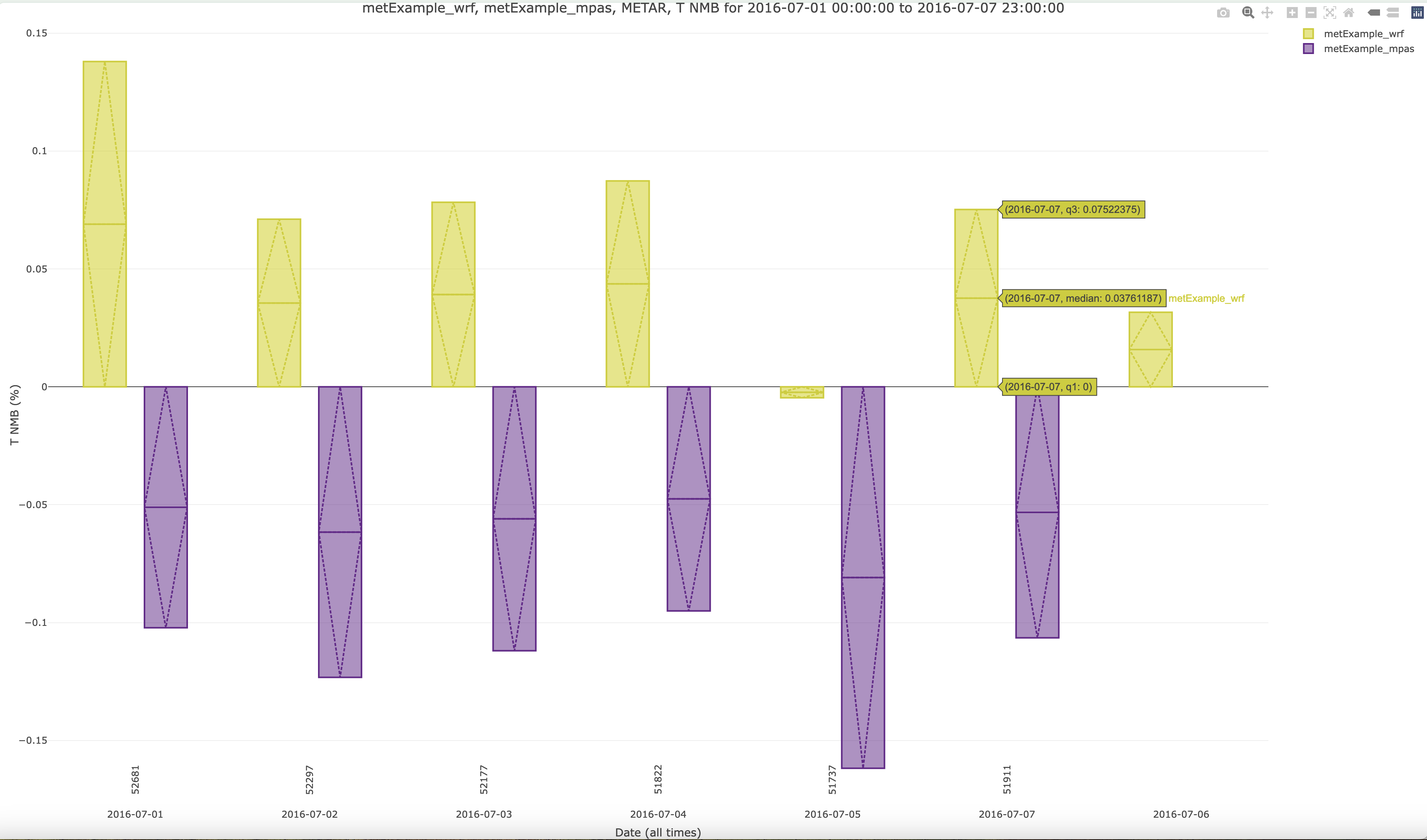
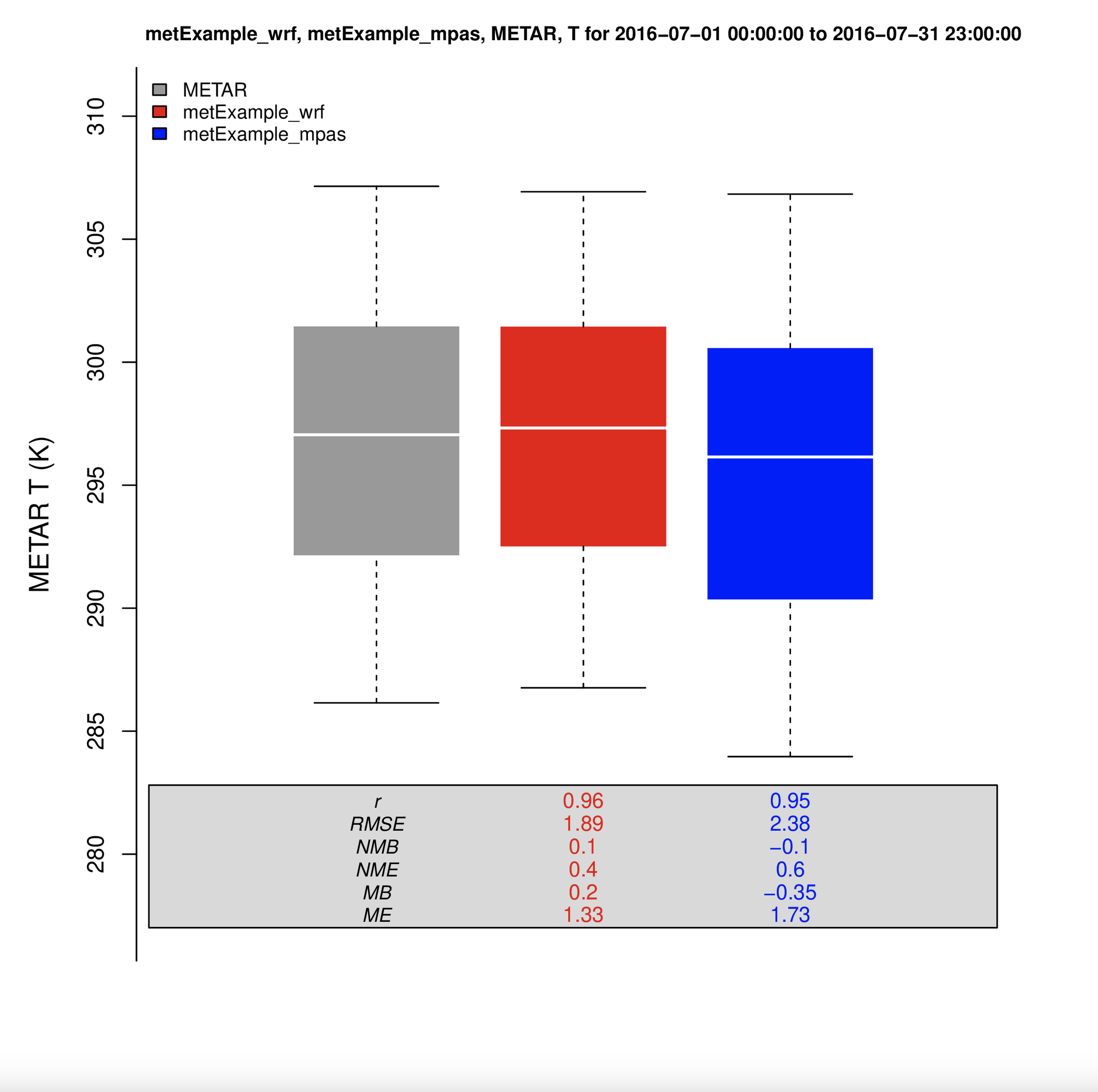
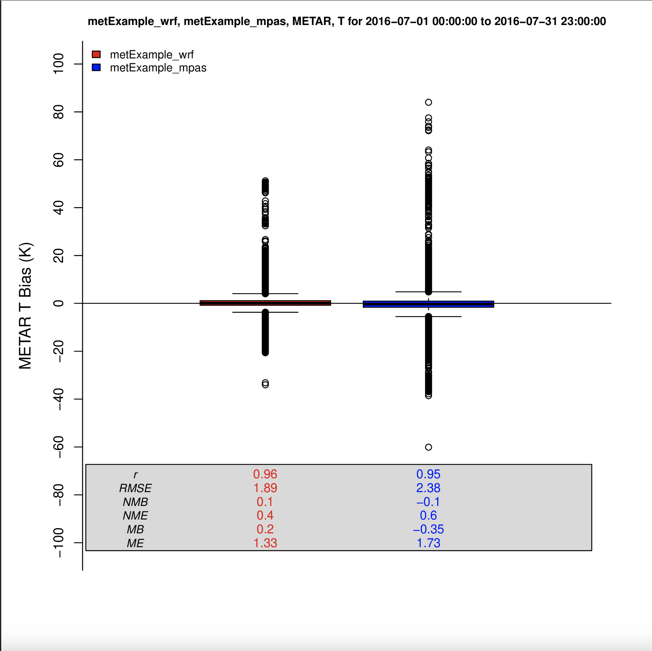
7.13.9. Create GGPlot Boxplot using METAR Met Observations and T(2m) Model Values

• Under Met Observation Networks
  • Choose METAR

• Under Met Variable to Use
  • Select T(2m)

• Under Date and Time Criteria select 1 week of data (full month of data is too crowded for this plot)
  • Select Start Date
  • Year: 2016
  • Month: 07
  • Day: 01
  • Select End Date
  • Year: 2016
  • Month: 07
  • Day: 07

• Under Choose Program to Run
  • GGPlot Boxplot (single network, multi-run)

Boxplot of T2 all

Boxplot of T2 Bias

7.13.10. Create Plotly Boxplot using METAR Met Observations and T(2m) Model Values

• Under Met Observation Networks
  • Choose METAR

• Under Met Variable to Use
  • Select T(2m)

• Under Date and Time Criteria select 1 week of data (this is one method to subset the time range, using an interactive plot, you can also grab a subset of the time region or a subset of the temperature range, which is demonstrated in the next Plotly interactive plot))
  • Select Start Date
  • Year: 2018
  • Month: 07
  • Day: 01
  • Select End Date
  • Year: 2018
  • Month: 07
  • Day: 07

• Under Choose Program to Run
  • Plotly Boxplot (single network, multi-run)

Plotly Boxplot of T2

Plotly Bias Plot of T2

Plotly NMB Plot of T2

7.13.11. Create Plotly Boxplot using METAR Met Observations and T(2m) Model Values for South Climate Region

• Under Climate Regions
  • Choose South

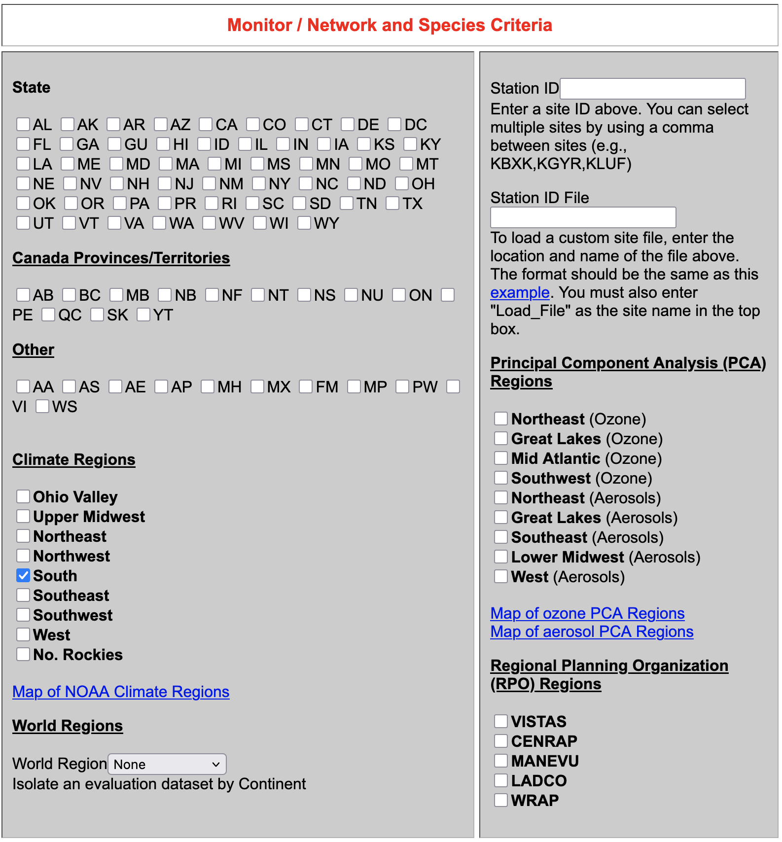
• Under Met Observation Networks
  • Choose METAR

• Under Met Variable to Use
  • Select T(2m)

• Under Date and Time Criteria select 1 month of data
  • Select Start Date
  • Year: 2018
  • Month: 07
  • Day: 01
  • Select End Date
  • Year: 2018
  • Month: 07
  • Day: 31

• Under Choose Program to Run
  • Plotly Boxplot (single network, multi-run)

Plotly Boxplot of T2 - this is an interactive plot, zoom in to show a smaller range of temperatures, 290K - 320K

Plotly Bias Plot of T2

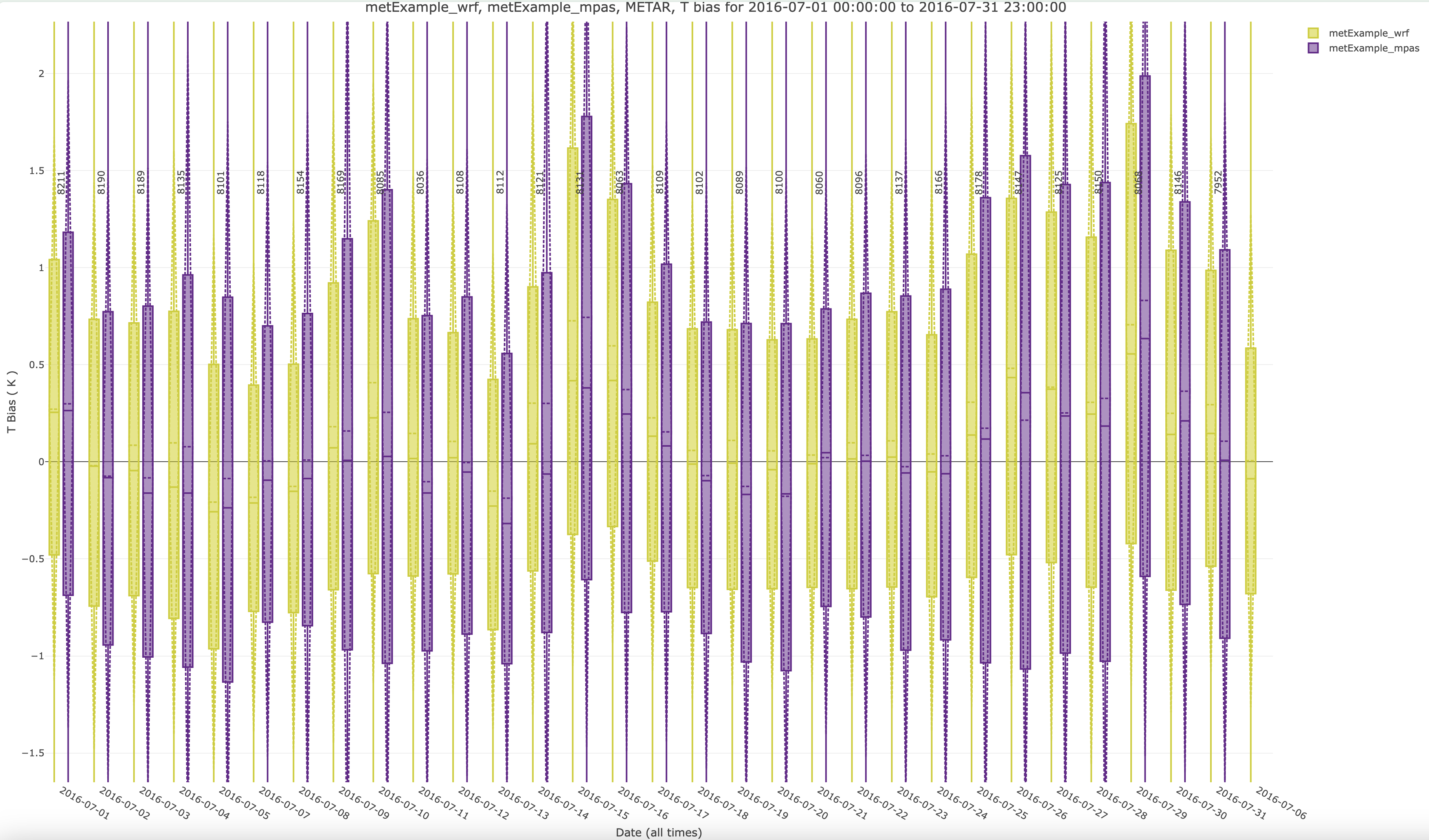
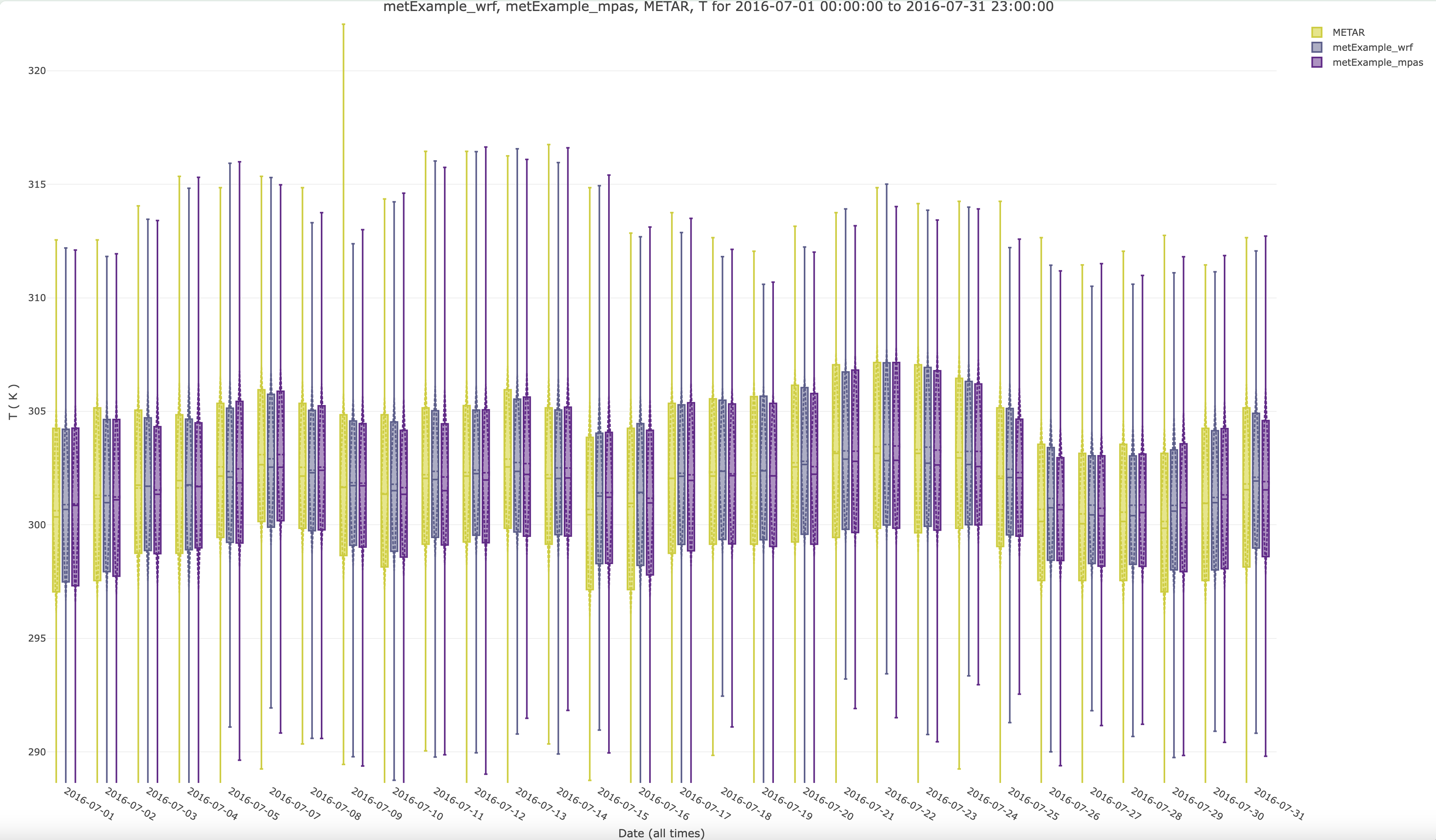
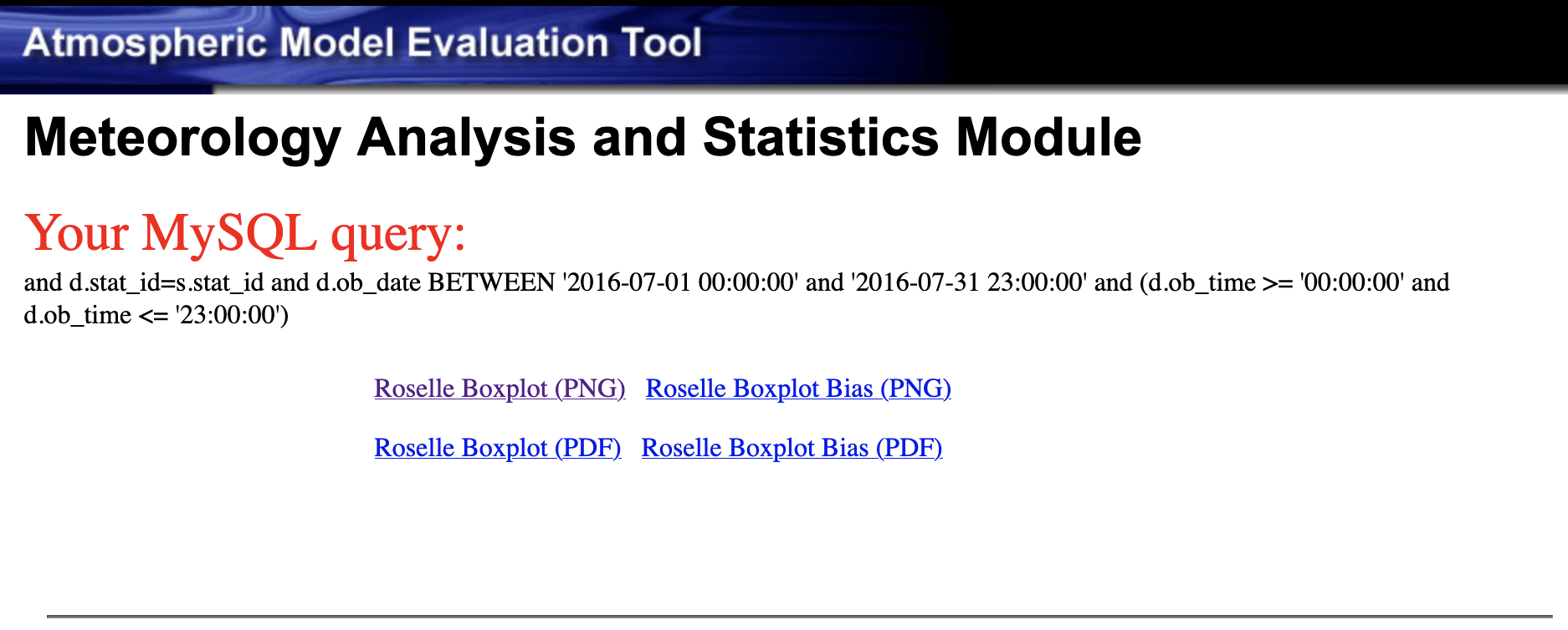
7.13.12. Create Roselle Boxplot

• Under Date and Time Criteria select 1 month of data
  • Select Start Date
  • Year: 2018
  • Month: 07
  • Day: 01
  • Select End Date
  • Year: 2018
  • Month: 07
  • Day: 31

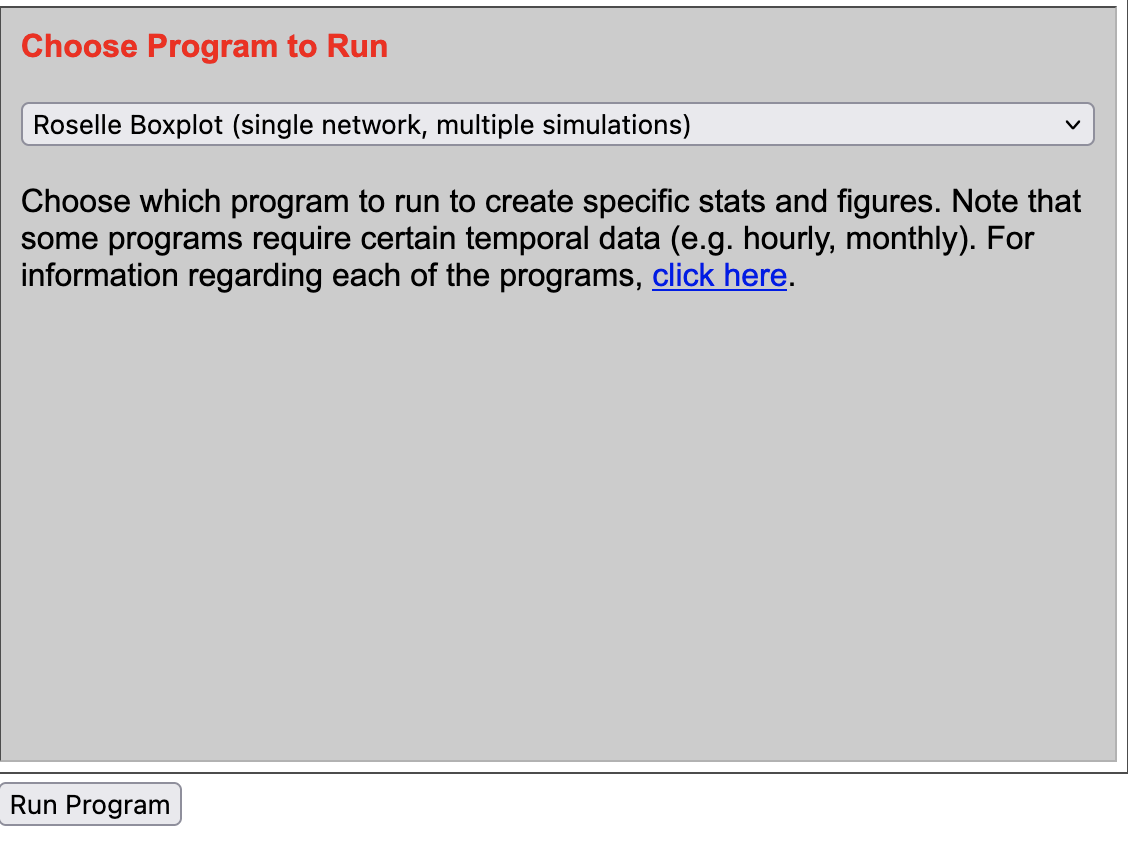
• Under Choose Program to Run
  • Roselle Boxplot (single network, multiple simulations)

Roselle Boxplot of T2

Roselle Bias Boxplot Plot of T2

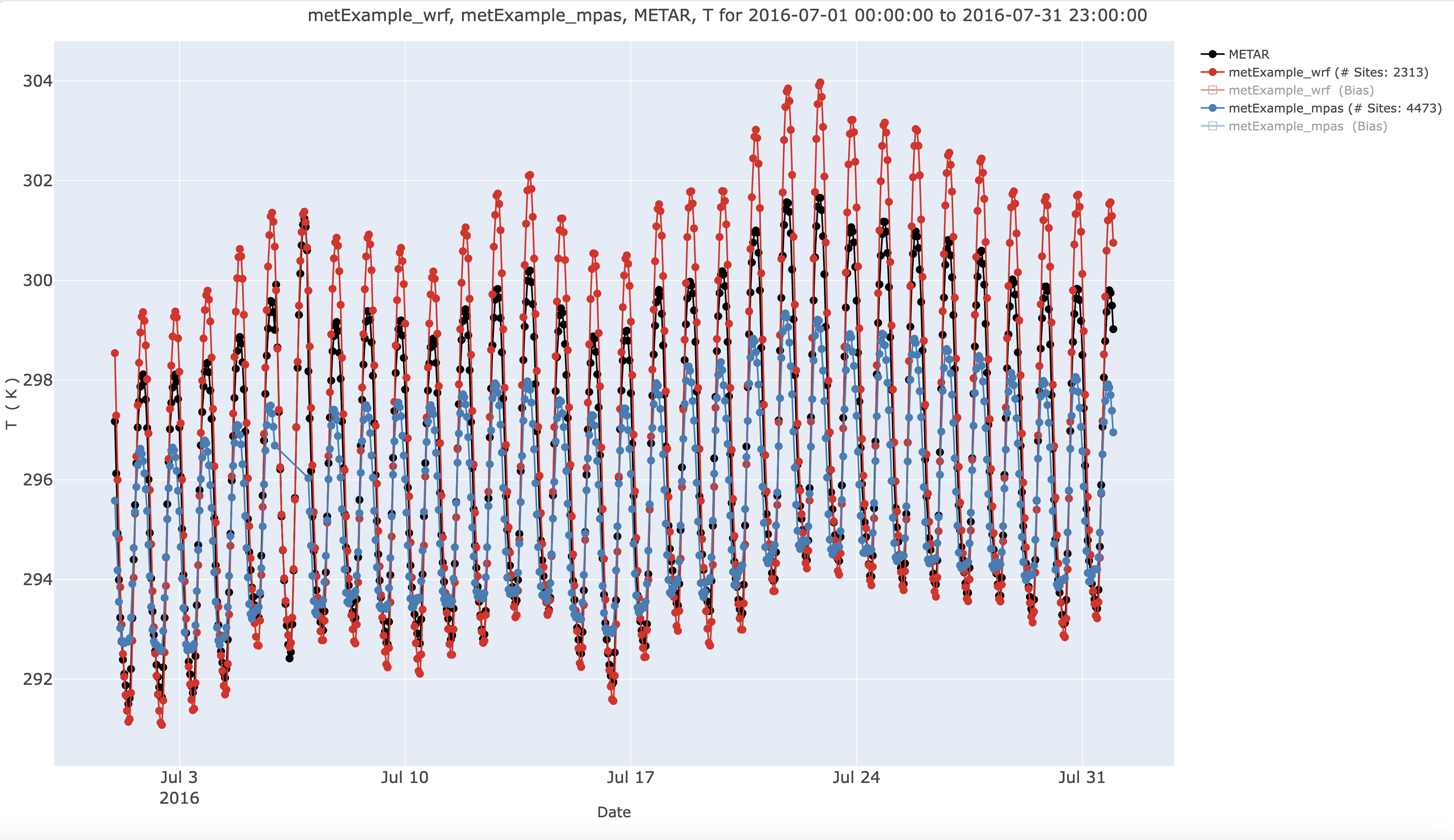
7.13.13. Create Interactive Hourly Timeseries of T2 using Plotly

• Under Met Observation Networks
  • Choose METAR

• Under Met Variable to Use
  • Select T(2m)

• Under Date and Time Criteria select 1 month of data
  • Select Start Date
  • Year: 2018
  • Month: 07
  • Day: 01
  • Select End Date
  • Year: 2018
  • Month: 07
  • Day: 31

• Under Choose Program to Run
  • Plotly Multi-species Timeseries

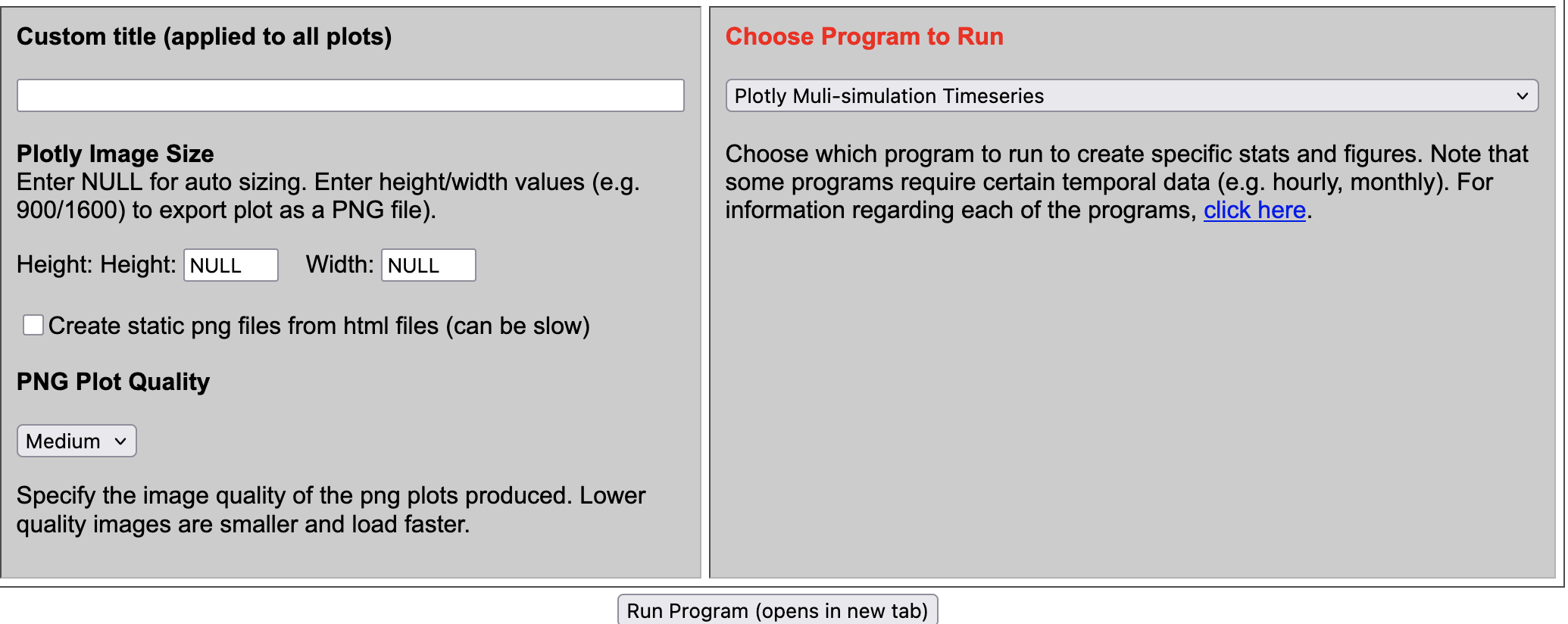
Note, this plot is interactive, and you can turn off items by clicking on an item in the legend, and also window to a specific time within the plot.

7.13.14. Create Interactive Hourly Timeseries of T2 using Plotly and select VISTAS RPO Region

• Under Met Observation Networks
  • Choose METAR

• Under Met Variable to Use
  • Select T(2m)

• Under Monitor / Network and Species Criteria
  • Select VISTAS RPO

• Under Date and Time Criteria select 1 month of data
  • Select Start Date
  • Year: 2018
  • Month: 07
  • Day: 01
  • Select End Date
  • Year: 2018
  • Month: 07
  • Day: 31

• Under Choose Program to Run
  • Plotly Multi-species Timeseries

Note, this plot is interactive, and you can turn off items by clicking on an item in the legend, and also window to a specific time within the plot.

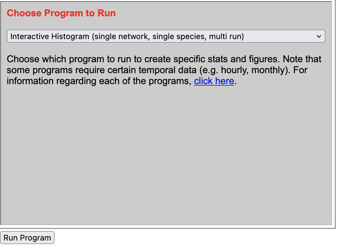
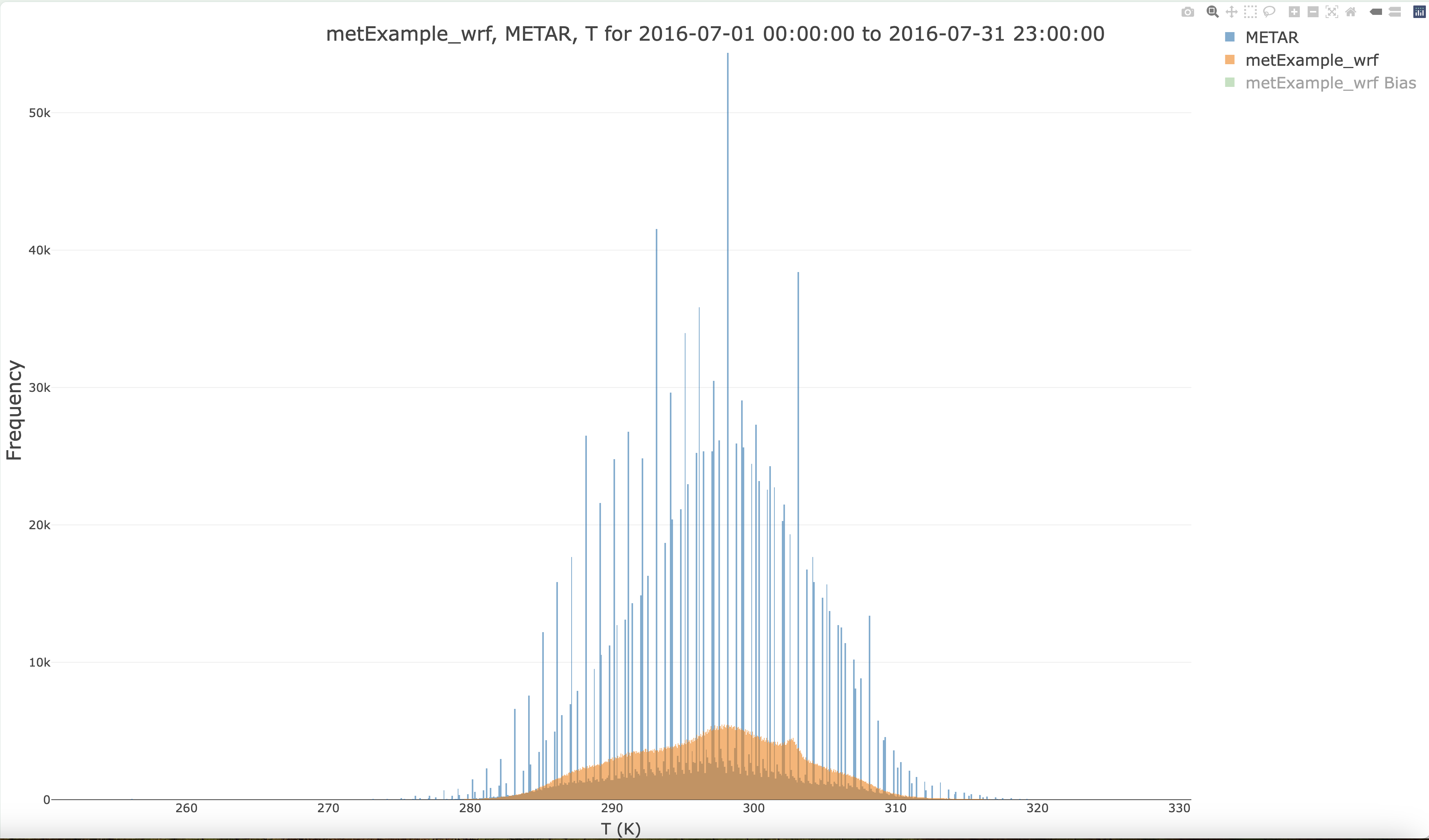
7.13.15. Create Histogram Plot of T(2m)

• Under Observation Network
  • Select METAR

• Under Met Species to Plot
  • Select T(2m)

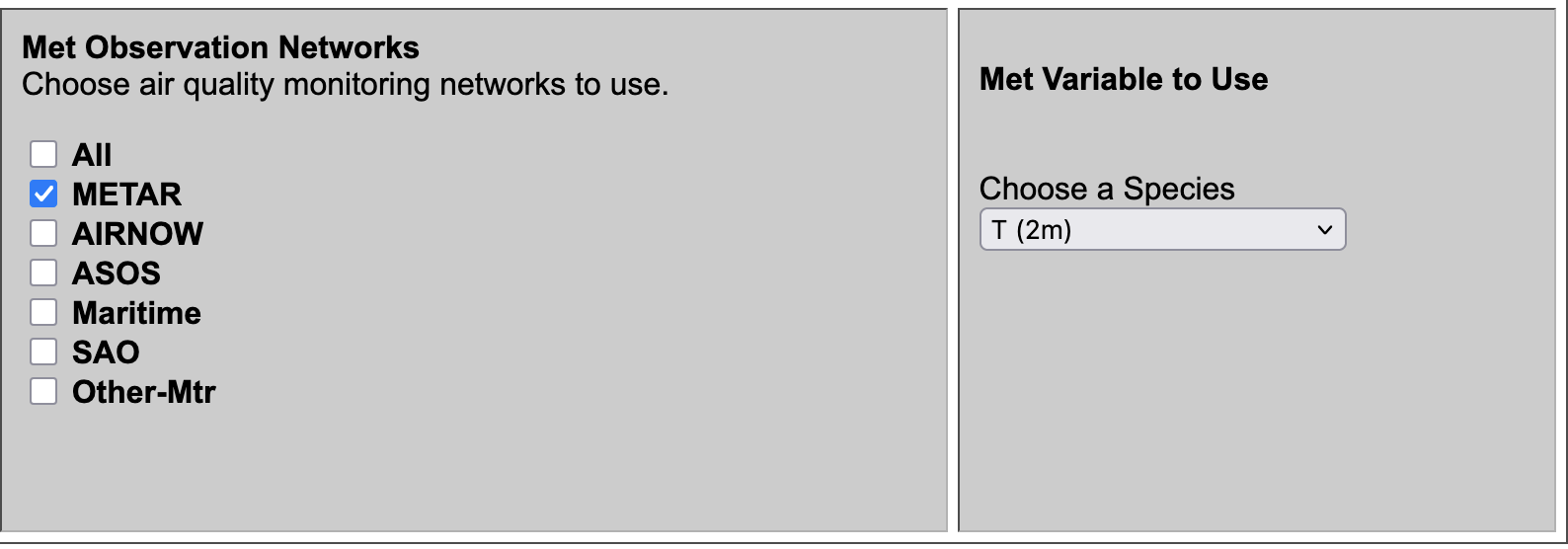
• Under Choose Program to Run
  • Interactive Histogram (single network, single species, multi-run) under Misc Scripts

Interactive Histogram Plot ( Frequency values for T and METAR Obs Network and for Bias)

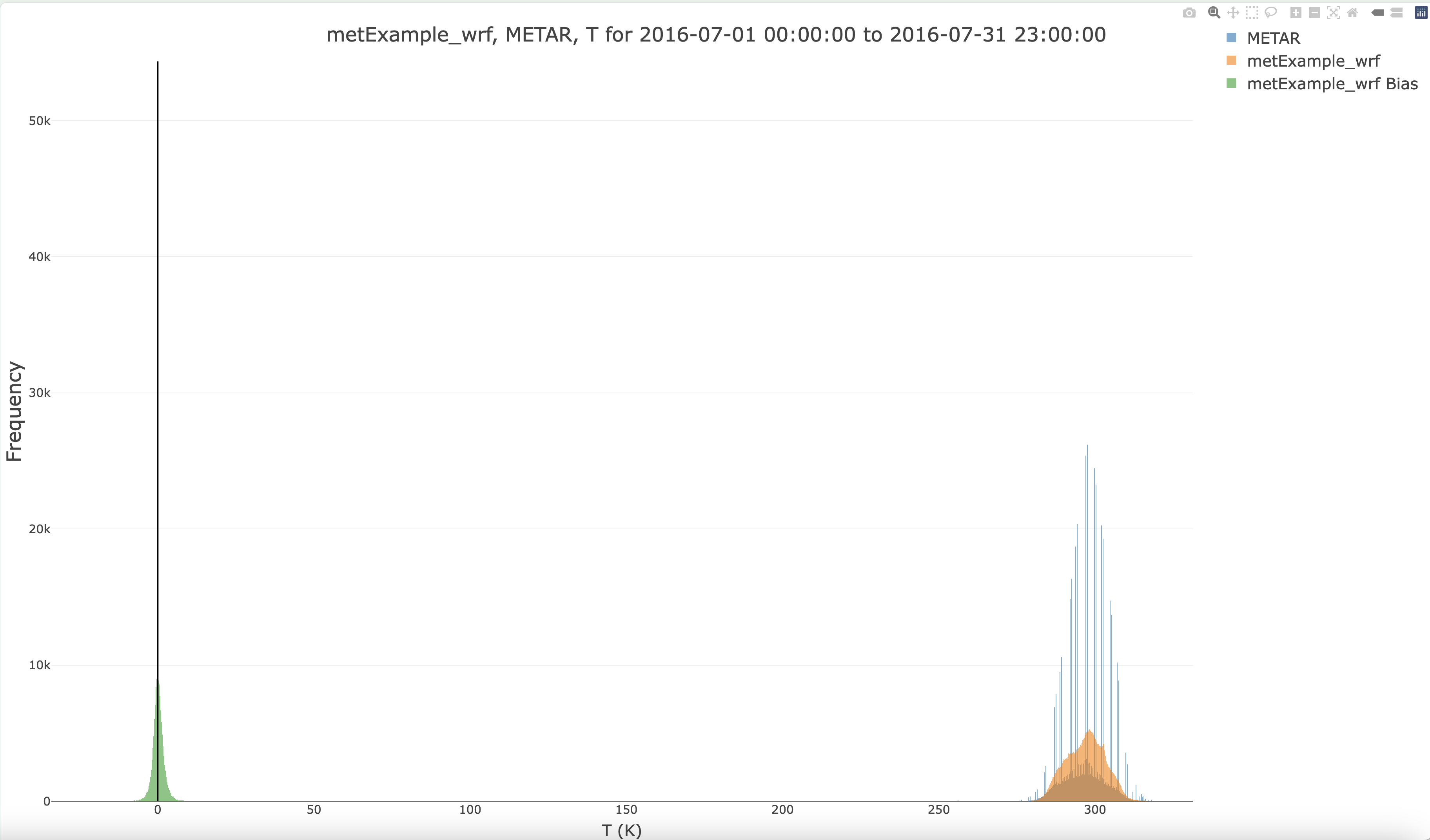
Turn off Bias by clicking in Legend, and zoom in to show frequency of temperature ranges for METAR and metExample_wrf

7.14. Load your own MET data to MariaDB

7.14.1. Prepare to load your own data

Load modules

Change to the c-shell

csh

Check modules available

module avail

Load Modules

module load ioapi-3.2/gcc-13.3  netcdf/gcc-13.3  openmpi/gcc  

Review directory set-up for files on /home/ubuntu

ls -lrt

total 48
drwxrwxr-x  3 ubuntu ubuntu 4096 Sep 23 16:43 Modules
drwxr-xr-x  3 ubuntu ubuntu 4096 Sep 23 18:15 aws
drwxrwxr-x 10 ubuntu ubuntu 4096 Sep 24 17:35 CMAQ55plus_REPO
drwxrwxr-x  8 ubuntu ubuntu 4096 Sep 24 17:52 CMAQv5.5+
drwx------  4 ubuntu ubuntu 4096 Sep 25 14:39 snap
drwxrwxr-x  3 ubuntu ubuntu 4096 Sep 25 17:17 MariaDB
drwxrwxrwx 15 ubuntu ubuntu 4096 Sep 25 19:30 AMET_v16
drwxrwxr-x  3 ubuntu ubuntu 4096 Sep 25 20:44 LIBRARIES
-rw-rw-r--  1 ubuntu ubuntu  467 Sep 29 17:25 ports.conf
-rw-rw-r--  1 ubuntu ubuntu 4962 Nov  3 15:22 branch_differences
-rw-rw-r--  1 ubuntu ubuntu  445 Nov  3 16:29 readme

Review directory set-up for files on /shared/AMET_v16

/shared/AMET_v16% ls -rlt */*
model_data/MET:
total 24
drwxrwxr-x 2 ubuntu ubuntu  4096 Sep 23 22:58 metExample_wrf
drwxrwxr-x 2 ubuntu ubuntu  4096 Sep 23 23:58 metExample_mpas
drwxrwxr-x 3 ubuntu ubuntu 12288 Sep 25 12:54 metExample_mcip

model_data/AQ:
total 4
drwxrwxr-x 2 ubuntu ubuntu   40 Nov  3 17:25 aqExample

Review size of data on /shared/AMET_v16 (note this is a 1 TB volume)

du -sh
768G

Review size of data on /home/ubuntu

du -sh
46G	.

Review size of the file systems available

df -h
Filesystem       Size  Used Avail Use% Mounted on
/dev/root        290G   61G  230G  21% /
tmpfs            7.8G     0  7.8G   0% /dev/shm
tmpfs            3.1G  1.0M  3.1G   1% /run
tmpfs            5.0M     0  5.0M   0% /run/lock
efivarfs         128K  4.1K  119K   4% /sys/firmware/efi/efivars
/dev/nvme0n1p16  881M  151M  669M  19% /boot
/dev/nvme0n1p15  105M  6.2M   99M   6% /boot/efi
/dev/nvme1n1    1000G  787G  214G  79% /shared
tmpfs            1.6G   20K  1.6G   1% /run/user/1000

Note that AMET_Website is installed under /var/www/html

ls -rlt /var/www/html
ubuntu@ip-172-31-30-106:/var/www/html/cache$ ls -rlt /var/www/html
total 1128
-rw-rw-r-- 1 www-data www-data   4333 Sep 23 17:55 AMET_Species_Name_Mapping.txt
-rw-rw-r-- 1 www-data www-data    420 Sep 23 17:55 example_stat_file.txt
-rw-rw-r-- 1 www-data www-data   2283 Sep 23 17:55 disaq_4km_met_sites.txt
-rw-rw-r-- 1 www-data www-data    331 Sep 23 17:55 disaq_1km_met_sites.txt
-rw-rw-r-- 1 www-data www-data   2700 Sep 23 17:55 O3_NA_monitors_2018.txt
-rw-rw-r-- 1 www-data www-data   8434 Sep 23 17:55 O3_NAA_Sites_v2_short_names.txt
-rw-rw-r-- 1 www-data www-data   4257 Sep 23 17:55 O3_NAA_Sites_v2_no_names.txt
drwxrwxr-x 2 www-data www-data   4096 Sep 23 17:55 images
-rw-rw-r-- 1 www-data www-data   6475 Sep 23 17:55 run_info_met.template
-rw-r--r-- 1 www-data www-data  10671 Sep 25 18:41 index.html.back
-rw-rw-r-- 1 www-data www-data    286 Sep 25 19:47 index.html.sv
-rw-rw-r-- 1 www-data www-data   3861 Oct 10 17:10 amet-lib.php
-rwxrwxr-x 1 www-data www-data   2061 Oct 10 17:24 amet-config.R
-rw-rw-r-- 1 www-data www-data  11397 Oct 10 17:30 run_info.template
-rw-rw-r-- 1 www-data www-data   2084 Nov 19 16:12 amet-www-config.php
-rwxrwxr-x 1 ubuntu   ubuntu   362779 Dec 11 17:59 querygen_aq.php
-rwxrwxr-x 1 ubuntu   ubuntu   259959 Jan 14 18:08 querygen_met.php
drwxrwxrwx 8 www-data www-data 425984 Mar  1 18:46 cache

7.14.2. Upload your own meteorology data

Change to the directory on /shared volume

cd /shared/AMET_v16/model_data/MET/ 
mkdir new_project

The wrfExample_mpas model data was 462 GB. The root volume of this AMI is only 500GB. Therefore, you will need to attach another 1 TB ebs volume to the EC2 instance if you needed to load model data for a new MPAS project.. The model data for the projects that have already been loaded into the database have been deleted as they are no longer needed.

See these instructions to attach a new volume. Instruction to attach EBS Volume to VM Instruction to use EBS Volume on AWS To load this data into the database, you will also need to change the EC2 instance type from t3.large to t3.2xlarge. Change instance type

use the s3 cp command to upload your data to the /shared/AMET_v16/model_data/MET/new_project directory

7.14.3. Load your project data into the database for a new MET project

Create a new project under the script_db directory

cd ~/AMET_v16/scripts_db/
cp -rp metExample_wrf new_project
cd new_project
mv matching_raob.csh new_project_matching_raob.csh

Modify the project name in the script

vi new_project_matching_raob.csh

Change:
  setenv AMET_PROJECT    metExample_wrf
to:
  setenv AMET_PROJECT    new_project

Edit the run description

Change:
 setenv RUN_DESCRIPTION "WRF release test dataset."
to
 setenv RUN_DESCRIPTION "WRF new project dataset."

Edit the path to the wrf output, if that is what you are uploading for your new_project.

Change:
setenv METOUTPUT $AMETBASE/model_data/MET/$AMET_PROJECT/wrfout_subset
to 
setenv METOUTPUT $AMETBASE/model_data/MET/$AMET_PROJECT/wrfout_new_project

7.15. Types of Errors Creating Plots and how to avoid them.

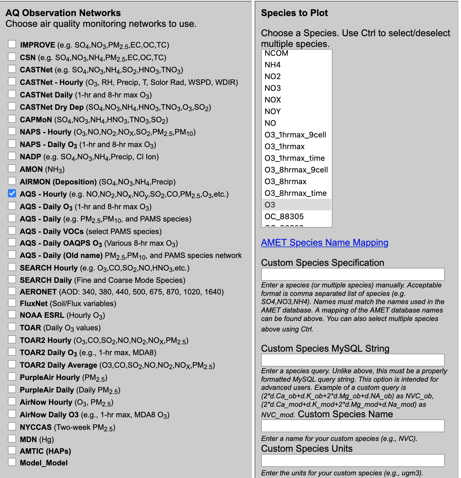
7.15.1. Selection of wrong inputs for the plot type selected to run

• Selection of O3 for AQS Daily, when AQS Daily only supports O3_8hrmax and O3_1hrmax)

  • Pay attention to the description in paranthesis next to the Obs Network name: AQS - Daily O3 (1-hr and 8-hr max O3)

  • In order for a plot to be generated, the observational network and the project (model output) must both contain species selected by the user for the same time range of interest.

• Date selection is automatically set for the first project, but if you add a second project, you need to change the data range to include that second project.

  • Pay attention to the dates selected!

• Selection of only one network for a plot program that is looking for multiple networks

  • Pay attention to the description in paranthesis next to the Program Name

7.15.2. Error due to missing data

• MetExample_mcip_surface didn’t load because the loop_over_days.csh script has that commented out, and the user needs to edit, link the required input files and rerun.

  • run a mysql query to verify that the data exists, or check your database loading logs

• Observation data not available to be loaded for specific networks, ie. METAR is the only network that appears to work for querygen_met.php

• Plots failed using CSN and IMPROVE with PM25_TOT but worked for AQS-Daily for the plotly multisimulation timeseries plot using the EQUATES database.

  • The amad_EQUATES database contains a limited subset of observational networks (AQS Daily, AQS Hourly, CASNET, and NADP)

• Observational data must be download and extracted for all of the years that correspondfor each project (model data), to enable obs/model pairing and loading into the database.

7.15.3. Bug or Error in the plot

• the legend symbols don’t match the data, or data isn’t plotted the way that the user expects.

• Bug - or error due to missing or mis-named program, search *.Rout for ‘Fatal Error’

7.15.4. Usability errors

• If programs are failing with a ‘Killed’ message, check to see if memory is being exceeded

  • login to the server and use htop to view the amount of memory/cpus being used

• consider upgrading the EC2 type to larger memory and cpus

• Error in loading the plot in the browser (browser slows down and asks if you want to stop the process) - plotly animated plots.

  • consider clearing your local browser cache

7.15.5. View error logs on the VM

cd /var/www/html/cache
ls *.Rout
tail AQ_Timeseries.Rout

Tail of Output:

+          }
+          #####################################
+       } # Close else statement
+    } # Close if/else statement
+ } # End num_runs loop
[1] "SELECT d.network,d.stat_id,s.lat,s.lon,LPAD(d.i,3,'0') as row,LPAD(d.j,3,'0') as col,d.ob_dates,d.ob_datee,d.ob_hour,d.month , d.NH4_ob, d.NH4_mod, d.precip_ob, d.precip_mod ,d.POCode,s.state,s.county from  aqExample  as d, site_metadata as s  WHERE d.NH4_ob is not NULL and d.network='NADP' and s.stat_id=d.stat_id and d.ob_dates BETWEEN 20180601 and 20180831 and d.ob_datee BETWEEN 20180601 and 20180831 and (d.ob_hour >= 00 and d.ob_hour <= 23)  and (d.valid_code = 't' or d.valid_code = 'd' or d.valid_code = 'w' or d.valid_code = 'wi' or d.valid_code = 'wd' or d.valid_code = 'wa') ORDER BY ob_dates,ob_hour"
Error in `$<-.data.frame`(`*tmp*`, "ob_hour", value = 0) : 
  replacement has 1 row, data has 0
Calls: query_dbase -> $<- -> $<-.data.frame
Execution halted

Note, that this query failed as there is no observational data loaded for the NADP network. (scroll to the right to see the full contents of the log file.)

7.15.6. Use the query by logging into the mysql database to understand what is missing

SELECT d.network,d.stat_id,s.lat,s.lon,LPAD(d.i,3,'0') as row,LPAD(d.j,3,'0') as col,d.ob_dates,d.ob_datee,d.ob_hour,d.month , d.SO4_ob, d.SO4_mod ,d.POCode,s.state,s.county from  aqExample  as d, site_metadata as s  WHERE (d.network='AQS_Hourly')  and s.stat_id=d.stat_id and d.ob_dates BETWEEN 20180601 and 20180831 and d.ob_datee BETWEEN 20180601 and 20180831 and (d.ob_hour >= 00 and d.ob_hour <= 23)  ORDER BY ob_dates,ob_hour limit 10;

Output

+------------+-----------+----------+------------+------+------+------------+------------+---------+-------+--------+---------+--------+-------+---------+
| network    | stat_id   | lat      | lon        | row  | col  | ob_dates   | ob_datee   | ob_hour | month | SO4_ob | SO4_mod | POCode | state | county  |
+------------+-----------+----------+------------+------+------+------------+------------+---------+-------+--------+---------+--------+-------+---------+
| AQS_Hourly | 060010007 | 37.68753 | -121.78422 | 148  | 035  | 2018-06-30 | 2018-06-30 |      16 |     6 |   NULL |    NULL | 1      | CA    | Alameda |
| AQS_Hourly | 060010007 | 37.68753 | -121.78422 | 148  | 035  | 2018-06-30 | 2018-06-30 |      16 |     6 |   NULL |    NULL | 3      | CA    | Alameda |
| AQS_Hourly | 060010007 | 37.68753 | -121.78422 | 148  | 035  | 2018-06-30 | 2018-06-30 |      16 |     6 |   NULL |    NULL | 6      | CA    | Alameda |
| AQS_Hourly | 060010009 | 37.74307 | -122.16993 | 149  | 032  | 2018-06-30 | 2018-06-30 |      16 |     6 |   NULL |    NULL | 1      | CA    | Alameda |
| AQS_Hourly | 060010009 | 37.74307 | -122.16993 | 149  | 032  | 2018-06-30 | 2018-06-30 |      16 |     6 |   NULL |    NULL | 3      | CA    | Alameda |
| AQS_Hourly | 060010011 | 37.81478 | -122.28235 | 150  | 032  | 2018-06-30 | 2018-06-30 |      16 |     6 |   NULL |    NULL | 1      | CA    | Alameda |
| AQS_Hourly | 060010011 | 37.81478 | -122.28235 | 150  | 032  | 2018-06-30 | 2018-06-30 |      16 |     6 |   NULL |    NULL | 3      | CA    | Alameda |
| AQS_Hourly | 060010012 | 37.79362 | -122.26338 | 150  | 032  | 2018-06-30 | 2018-06-30 |      16 |     6 |   NULL |    NULL | 1      | CA    | Alameda |
| AQS_Hourly | 060010012 | 37.79362 | -122.26338 | 150  | 032  | 2018-06-30 | 2018-06-30 |      16 |     6 |   NULL |    NULL | 3      | CA    | Alameda |
| AQS_Hourly | 060010013 | 37.86477 | -122.30274 | 150  | 032  | 2018-06-30 | 2018-06-30 |      16 |     6 |   NULL |    NULL | 1      | CA    | Alameda |
+------------+-----------+----------+------------+------+------+------------+------------+---------+-------+--------+---------+--------+-------+---------+
10 rows in set (59.217 sec)

SELECT d.network,d.stat_id,s.lat,s.lon,LPAD(d.i,3,'0') as row,LPAD(d.j,3,'0') as col,d.ob_dates,d.ob_datee,d.ob_hour,d.month , d.SO4_ob, d.SO4_mod ,d.POCode,s.state,s.county from  aqExample  as d, site_metadata as s  WHERE (d.network='NADP')  and s.stat_id=d.stat_id and d.ob_dates BETWEEN 20180601 and 20180831 and d.ob_datee BETWEEN 20180601 and 20180831 and (d.ob_hour >= 00 and d.ob_hour <= 23)  ORDER BY ob_dates,ob_hour limit 10;

Output:

+---------+---------+---------+-----------+------+------+------------+------------+---------+-------+--------+---------+--------+-------+------------+
| network | stat_id | lat     | lon       | row  | col  | ob_dates   | ob_datee   | ob_hour | month | SO4_ob | SO4_mod | POCode | state | county     |
+---------+---------+---------+-----------+------+------+------------+------------+---------+-------+--------+---------+--------+-------+------------+
| NADP    | SK20    | 52.0223 | -109.8616 | 262  | 139  | 2018-06-30 | 2018-07-31 |      17 |     7 |   NULL |    NULL | 1      | SK    | -999       |
| NADP    | SD08    | 43.9461 | -101.8552 | 182  | 181  | 2018-06-30 | 2018-07-31 |      17 |     7 |   NULL |    NULL | 1      | SD    | Jackson    |
| NADP    | GA20    | 32.0849 |  -81.9367 | 081  | 331  | 2018-06-30 | 2018-07-31 |      19 |     7 |   NULL |    NULL | 1      | GA    | Evans      |
| NADP    | PA42    | 40.6575 |  -77.9397 | 164  | 346  | 2018-07-02 | 2018-07-09 |       4 |     7 |   NULL |    NULL | 1      | PA    | Huntingdon |
| NADP    | WY99    |  43.873 | -104.1917 | 182  | 166  | 2018-07-02 | 2018-07-10 |       6 |     7 |   NULL |    NULL | 1      | WY    | Weston     |
| NADP    | ME94    | 45.2436 |  -67.6308 | 224  | 402  | 2018-07-02 | 2018-07-10 |       7 |     7 |   NULL |    NULL | 1      | ME    | Washington |
| NADP    | NY10    | 42.2994 |  -79.3964 | 177  | 333  | 2018-07-02 | 2018-07-10 |       7 |     7 |   NULL |    NULL | 1      | NY    | Chautauqua |
| NADP    | ME00    | 46.8675 |  -68.0134 | 237  | 395  | 2018-07-02 | 2018-07-10 |      12 |     7 |   NULL |    NULL | 1      | ME    | Aroostook  |
| NADP    | SD04    | 43.5577 |  -103.484 | 179  | 170  | 2018-07-02 | 2018-07-10 |      13 |     7 |   NULL |    NULL | 1      | SD    | Custer     |
| NADP    | WA24    | 46.7606 | -117.1847 | 221  | 086  | 2018-07-02 | 2018-07-10 |      14 |     7 |   NULL |    NULL | 1      | WA    | Whitman    |
+---------+---------+---------+-----------+------+------+------------+------------+---------+-------+--------+---------+--------+-------+------------+
10 rows in set (0.036 sec)

select * from aqExample where network='AQS_Daily' limit 2;

Output

| proj_code | POCode | valid_code | invalid_code | replicate | network   | stat_id   | stat_id_POCode | lat     | lon      | i    | j    | ob_dates   | ob_datee   | ob_hour | month | precip_ob | precip_mod | SO4_ob | SO4_mod | NO3_ob | NO3_mod   | NH4_ob | NH4_mod  | PM_TOT_ob | PM_TOT_mod | OC_ob | OC_mod  | EC_ob | EC_mod   | TC_ob | TC_mod  | Cl_ob | Cl_mod    | PM10_IJK_ob | PM10_IJK_mod | PMC_TOT_ob | PMC_TOT_mod | PM25_SO4_ob | PM25_SO4_mod | PM25_NO3_ob | PM25_NO3_mod | PM25_NH4_ob | PM25_NH4_mod | PM25_OC_ob | PM25_OC_mod | PM25_EC_ob | PM25_EC_mod | PM25_TC_ob | PM25_TC_mod | PM25_TOT_ob | PM25_TOT_mod | PM10_ob | PM10_mod | PM25_Cl_ob | PM25_Cl_mod | PMC_TOT_CUT_ob | PMC_TOT_CUT_mod | Na_ob | Na_mod   | NaCl_ob | NaCl_mod | Fe_ob | Fe_mod   | Al_ob | Al_mod    | Si_ob | Si_mod   | Ti_ob | Ti_mod     | Ca_ob | Ca_mod   | Mg_ob | Mg_mod    | K_ob | K_mod    | Mn_ob | Mn_mod     | soil_ob | soil_mod | OTHER_ob | OTHER_mod | NCOM_ob | NCOM_mod | OTHER_REM_ob | OTHER_REM_mod | PM_TOT_88101_ob | PM_TOT_88101_mod | PM_TOT_88502_ob | PM_TOT_88502_mod | OC_88305_ob | OC_88305_mod | OC_88305_adj_ob | OC_88305_adj_mod | OC_88370_ob | OC_88370_mod | OC_88370_adj_ob | OC_88370_adj_mod | OC_88320_ob | OC_88320_mod | EC_88307_ob | EC_88307_mod | EC_88307_adj_ob | EC_88307_adj_mod | EC_88380_ob | EC_88380_mod | EC_88321_ob | EC_88321_mod | TNO3_ob | TNO3_mod | SO4_IJK_ob | SO4_IJK_mod | NO3_IJK_ob | NO3_IJK_mod | NH4_IJK_ob | NH4_IJK_mod | TNO3_IJK_ob | TNO3_IJK_mod | PM25_TNO3_ob | PM25_TNO3_mod | MG_JK_ob | MG_JK_mod | CA_JK_ob | CA_JK_mod | K_JK_ob | K_JK_mod | CL_PMC_ob | CL_PMC_mod | NA_PMC_ob | NA_PMC_mod | NA_IJK_ob | NA_IJK_mod | HNO3_ob | HNO3_mod | SO2_ob | SO2_mod | SO2_adj_ob | SO2_adj_mod | O3_ob | O3_mod | SFC_TMP_ob | SFC_TMP_mod | RH_ob | RH_mod | Solar_Rad_ob | Solar_Rad_mod | WSPD10_ob | WSPD10_mod | O3_1hrmax_ob | O3_1hrmax_mod | O3_1hrmax_9cell_ob | O3_1hrmax_9cell_mod | O3_1hrmax_time_ob | O3_1hrmax_time_mod | O3_8hrmax_ob | O3_8hrmax_mod | O3_8hrmax_9cell_ob | O3_8hrmax_9cell_mod | O3_8hrmax_time_ob | O3_8hrmax_time_mod | W126_ob | W126_mod | SUM06_ob | SUM06_mod | SO2_ddep_ob | SO2_ddep_mod | HNO3_ddep_ob | HNO3_ddep_mod | TNO3_ddep_ob | TNO3_ddep_mod | SO4_ddep_ob | SO4_ddep_mod | NO3_ddep_ob | NO3_ddep_mod | NH4_ddep_ob | NH4_ddep_mod | O3_ddep_ob | O3_ddep_mod | NH4_dep_ob | NH4_dep_mod | NO3_dep_ob | NO3_dep_mod | SO4_dep_ob | SO4_dep_mod | Cl_dep_ob | Cl_dep_mod | Na_dep_ob | Na_dep_mod | CA_dep_ob | CA_dep_mod | MG_dep_ob | MG_dep_mod | K_dep_ob | K_dep_mod | NH4_conc_ob | NH4_conc_mod | NO3_conc_ob | NO3_conc_mod | SO4_conc_ob | SO4_conc_mod | Cl_conc_ob | Cl_conc_mod | Na_conc_ob | Na_conc_mod | CA_conc_ob | CA_conc_mod | MG_conc_ob | MG_conc_mod | K_conc_ob | K_conc_mod | PM_FRM_ob | PM_FRM_mod | Isoprene_ob | Isoprene_mod | Ethylene_ob | Ethylene_mod | Ethane_ob | Ethane_mod | Toluene_ob | Toluene_mod | Acetaldehyde_ob | Acetaldehyde_mod | Formaldehyde_ob | Formaldehyde_mod | Benzene_ob | Benzene_mod | TC_88305_ob | TC_88305_mod | TC_88370_ob | TC_88370_mod | EC_88320_ob | EC_88320_mod | TC_88320_ob | TC_88320_mod | PM25_OC_88305_ob | PM25_OC_88305_mod | PM25_EC_88307_ob | PM25_EC_88307_mod | PM25_TC_88305_ob | PM25_TC_88305_mod | PM25_OC_88370_ob | PM25_OC_88370_mod | PM25_EC_88380_ob | PM25_EC_88380_mod | PM25_TC_88370_ob | PM25_TC_88370_mod | PM25_OC_88320_ob | PM25_OC_88320_mod | PM25_EC_88321_ob | PM25_EC_88321_mod | PM25_TC_88320_ob | PM25_TC_88320_mod | CO_ob | CO_mod | NO_ob | NO_mod | NO2_ob | NO2_mod | NOX_ob | NOX_mod | NOY_ob | NOY_mod | PBLH_mod |

SELECT d.network,d.stat_id,s.lat,s.lon,LPAD(d.i,3,'0') as row,LPAD(d.j,3,'0') as col,d.ob_dates,d.ob_datee,d.ob_hour,d.month , d.NO_ob, d.NO_mod ,d.POCode,s.state,s.county from  aqExample  as d, site_metadata as s  WHERE (d.network='AQS_Hourly')  and s.stat_id=d.stat_id and d.ob_dates BETWEEN 20180601 and 20180831 and d.ob_datee BETWEEN 20180601 and 20180831 and (d.ob_hour >= 00 and d.ob_hour <= 23)  ORDER BY ob_dates,ob_hour limit 10;

Output:

+------------+-----------+----------+------------+------+------+------------+------------+---------+-------+-------+---------+--------+-------+---------+
| network    | stat_id   | lat      | lon        | row  | col  | ob_dates   | ob_datee   | ob_hour | month | NO_ob | NO_mod  | POCode | state | county  |
+------------+-----------+----------+------------+------+------+------------+------------+---------+-------+-------+---------+--------+-------+---------+
| AQS_Hourly | 060010007 | 37.68753 | -121.78422 | 148  | 035  | 2018-06-30 | 2018-06-30 |      16 |     6 |   0.2 | 0.32431 | 1      | CA    | Alameda |
| AQS_Hourly | 060010007 | 37.68753 | -121.78422 | 148  | 035  | 2018-06-30 | 2018-06-30 |      16 |     6 |  -999 | 0.32431 | 3      | CA    | Alameda |
| AQS_Hourly | 060010007 | 37.68753 | -121.78422 | 148  | 035  | 2018-06-30 | 2018-06-30 |      16 |     6 |  -999 | 0.32431 | 6      | CA    | Alameda |
| AQS_Hourly | 060010009 | 37.74307 | -122.16993 | 149  | 032  | 2018-06-30 | 2018-06-30 |      16 |     6 |     2 |  1.2824 | 1      | CA    | Alameda |
| AQS_Hourly | 060010009 | 37.74307 | -122.16993 | 149  | 032  | 2018-06-30 | 2018-06-30 |      16 |     6 |  -999 |  1.2824 | 3      | CA    | Alameda |
| AQS_Hourly | 060010011 | 37.81478 | -122.28235 | 150  | 032  | 2018-06-30 | 2018-06-30 |      16 |     6 |   1.2 |  2.4289 | 1      | CA    | Alameda |
| AQS_Hourly | 060010011 | 37.81478 | -122.28235 | 150  | 032  | 2018-06-30 | 2018-06-30 |      16 |     6 |  -999 |  2.4289 | 3      | CA    | Alameda |
| AQS_Hourly | 060010012 | 37.79362 | -122.26338 | 150  | 032  | 2018-06-30 | 2018-06-30 |      16 |     6 |   1.2 |  2.4289 | 1      | CA    | Alameda |
| AQS_Hourly | 060010012 | 37.79362 | -122.26338 | 150  | 032  | 2018-06-30 | 2018-06-30 |      16 |     6 |  -999 |  2.4289 | 3      | CA    | Alameda |
| AQS_Hourly | 060010013 | 37.86477 | -122.30274 | 150  | 032  | 2018-06-30 | 2018-06-30 |      16 |     6 |   6.9 |  2.4289 | 1      | CA    | Alameda |
+------------+-----------+----------+------------+------+------+------------+------------+---------+-------+-------+---------+--------+-------+---------+